



What Steel Fatigue Properties Actually Describe
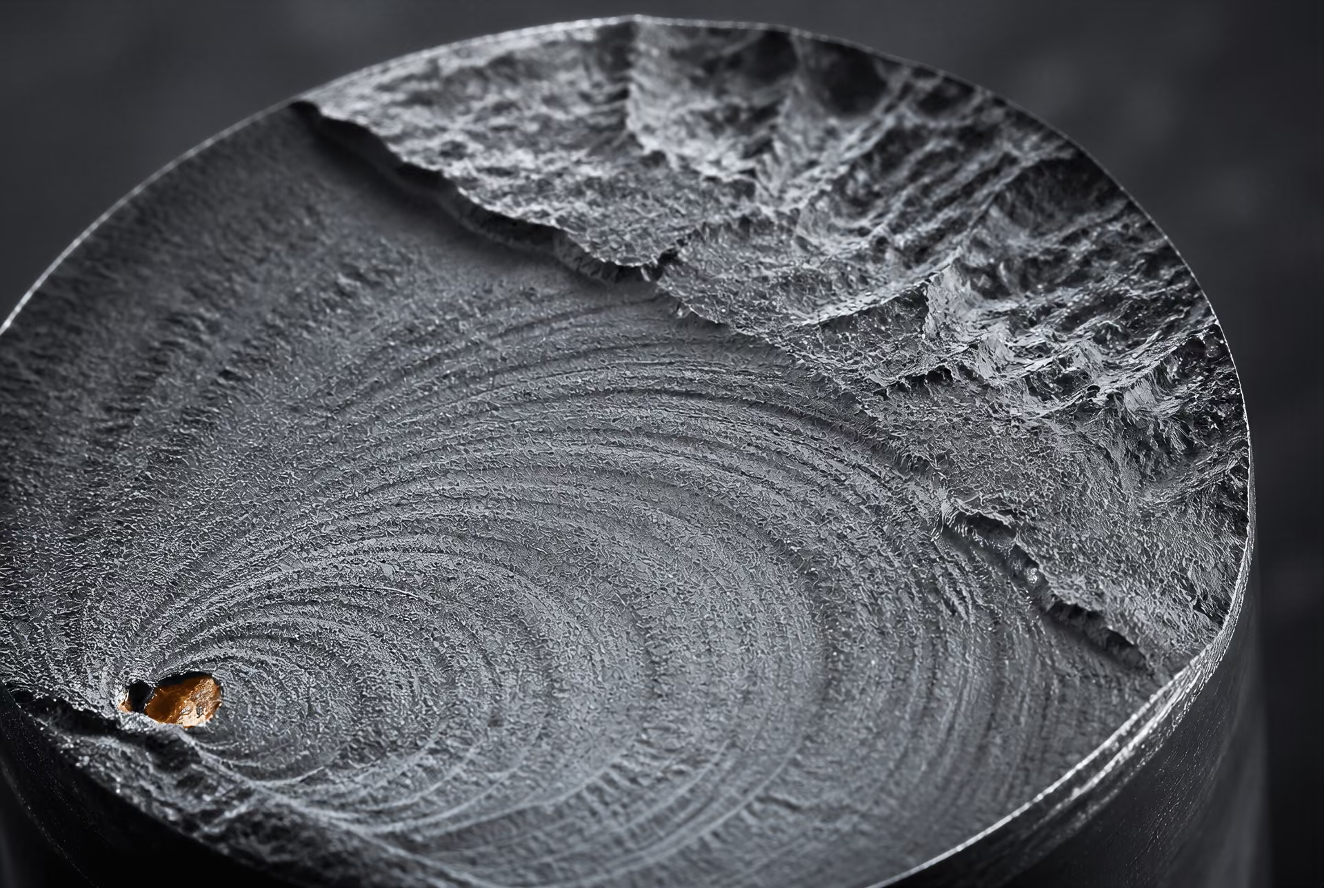
Fatigue is progressive damage caused by repeated or fluctuating loading. A steel part can withstand a static load below its tensile capacity and still fail after thousands, millions, or billions of cycles. Each cycle may cause only a minute increment of plasticity, slip, crack growth, or damage at a surface, notch, inclusion, or weld toe. The accumulated effect is fatigue failure.
Fatigue life, fatigue strength, and failure definition
Fatigue life is the number of load cycles associated with a defined event. That event must be stated, because “failure” does not always mean the same thing in a fatigue test or design calculation. Some tests count cycles to complete fracture. Others stop when a crack reaches a specified length, when stiffness falls by a set percentage, or when the specimen can no longer carry the applied force.

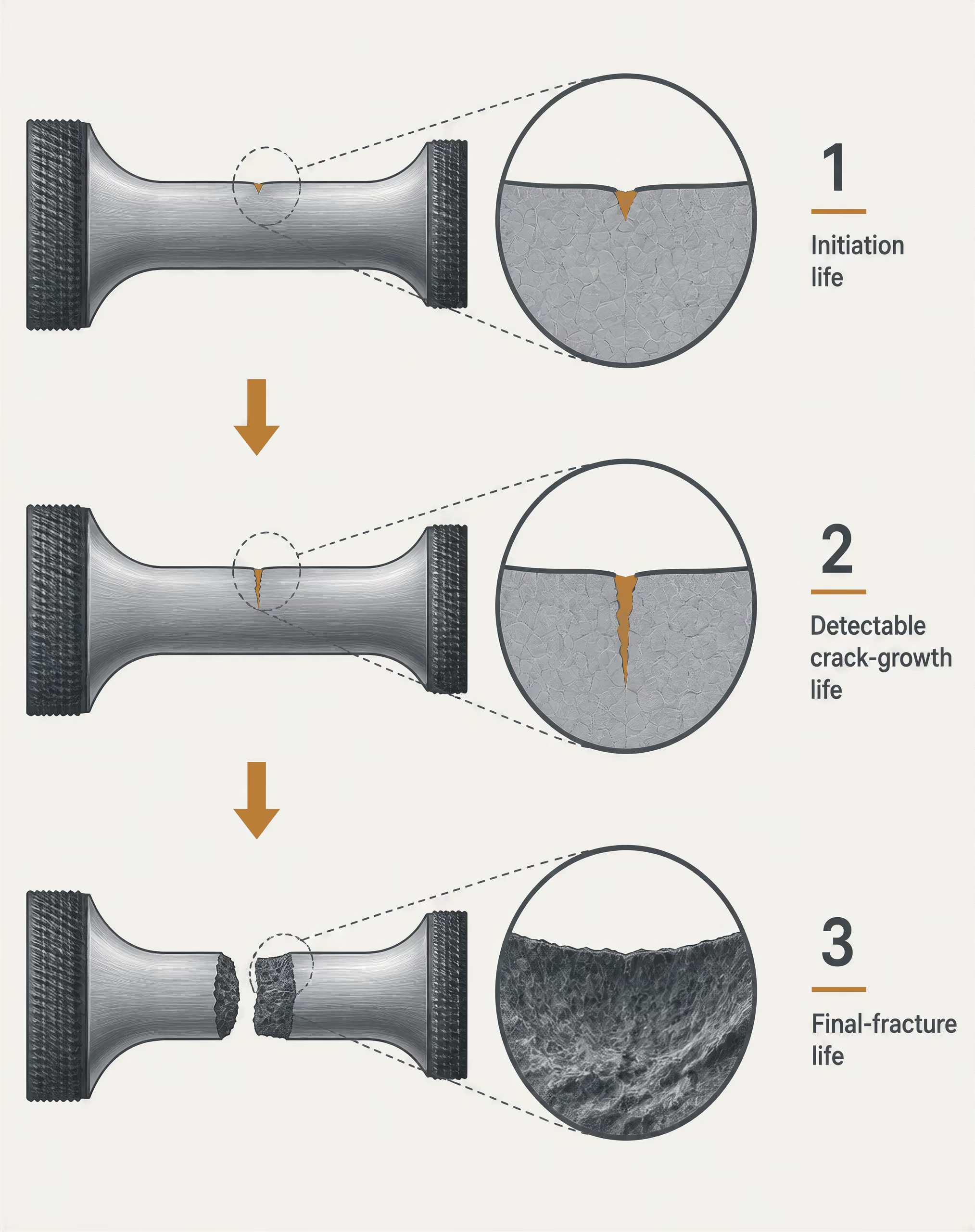
Three stages of fatigue life
- Crack initiation life Cycles required to form a crack of a specified size, often at a surface or stress concentration.
- Detectable crack-growth life Cycles from the initial crack condition until inspection can identify the crack or it reaches a defined length.
- Final-fracture life Cycles from detected cracking to unstable fracture or loss of required load-carrying capacity.
A useful distinction is between three stages:
1. Crack initiation life: cycles required to form a crack of a specified size, often at a surface or stress concentration. 2. Detectable crack-growth life: cycles from that condition until inspection can reliably identify the crack, or until it reaches a defined length. 3. Final-fracture life: cycles from the detected crack to unstable fracture or loss of the required load-carrying capacity.
A polished laboratory specimen may contain no deliberately introduced crack, so its reported life can include initiation and propagation. A fracture-mechanics assessment may begin with an assumed flaw and calculate only propagation. Those results are not interchangeable.
Fatigue strength is the stress level associated with a specified fatigue life and failure criterion. For example, a test might report the stress range producing failure at cycles. An endurance limit is a narrower claim: it is a stress level below which the chosen specimen is expected not to fail within the tested or defined life range. It is not automatically a permanent property of every part made from that steel.
The stress–life method expresses stress amplitude or stress range against cycles to failure, commonly through a Basquin-type power law. The Federal Highway Administration describes steel S–N curves as plots of stress range versus cycles to failure on logarithmic axes. ISO 1099:2017 specifies ambient-temperature, constant-amplitude, axial force-controlled testing at stated stress ratios. ASTM E466-21 covers force-controlled, constant-amplitude axial loading of unnotched and notched metallic specimens in air at room temperature. These conditions define the result.
Stress ratio matters because the minimum and maximum stresses affect crack opening, plasticity, and mean-stress effects. A cycle between zero and tension is not equivalent to a fully reversed cycle, even when the stress amplitude is identical. Loading frequency, temperature, corrosion, and waveform can also change the measured life.
Why cyclic stress is different from static strength
Yield strength and tensile strength describe resistance under particular monotonic loading conditions. They do not, by themselves, determine fatigue performance. Two steels with similar yield strength can produce different S–N curves because of differences in cleanliness, inclusions, heat treatment, grain structure, residual stress, surface condition, or crack-growth behavior. Conversely, increasing strength does not guarantee a proportional increase in fatigue life when the controlling defect is a weld toe, corrosion pit, machining mark, or other notch.
| Material or detail | What the designation identifies | Why it does not alone predict fatigue life |
|---|---|---|
| ASTM A36 steel | Specified grade and strength requirements | A welded detail may be governed by weld profile and residual stress |
| ASTM A572/A572M Grade 50 steel | Specified higher-strength structural grade | Nominal strength does not define notch, surface, weld, or corrosion effects |
| ASTM A514/A514M plate | Quenched-and-tempered high-strength plate | High strength does not guarantee proportional fatigue-life improvement |
Grade designations illustrate the limitation. ASTM A36 steel, ASTM A572/A572M Grade 50 steel, and quenched-and-tempered ASTM A514/A514M plate have different specified strength levels and metallurgical conditions, but a welded detail may be governed more by weld profile and residual stress than by the parent plate’s nominal yield strength. In a welded connection, the fatigue category generally relates to the detail configuration, weld geometry, direction of stress, and likely crack location.
At low and moderate cycle counts, cyclic plastic strain may dominate, making a strain–life method more suitable than a stress–life curve. At high cycle counts, nominal stress can remain below yield while local stress at a notch exceeds the elastic estimate. Fatigue therefore concerns repeated local damage, not simply whether the gross section has yielded once.
The apparent endurance limit also depends on the cycle range examined. The 2019 review The gigacycle fatigue strength of steels: a review of structural and operating factors reports that low-strength steels often show an approximately horizontal S–N asymptote, while high-strength steels can show a second decline beyond about cycles. A curve that appears flat through cycles should not automatically be extended to cycles.
Material data versus component and detail data
A material S–N curve is baseline data for a specified specimen, processing condition, geometry, environment, loading type, stress ratio, and failure definition. It is conditional evidence, not an immutable grade-wide constant. ASTM E466-21 permits both unnotched and notched specimens, but the resulting curves describe those tested configurations.
A real component adds size effects, surface finish, residual stress, holes, threads, contact loads, misalignment, local stress concentration, temperature, and corrosion. A smooth, polished coupon tested in laboratory air cannot be transferred without qualification to a corroded shaft, a machined notch, or a bridge attachment with a welded toe.
Design data are often detail-specific. The Steel Construction Institute’s 2018 NSC Technical Digest describes fatigue assessment using curves for plain-steel members, welded joints, and welded attachments, with cumulative damage summed linearly for a given detail under a specified loading spectrum. For welded steel details, the AISC bridge-fatigue manual places design S–N curves two standard deviations below the logarithmic mean fatigue-life data, corresponding to approximately 97.5% survival. That statistical lower bound is a design choice, not a new metallurgical property.
Variable-amplitude service loading introduces another distinction. A component may experience occasional high stress ranges among many smaller cycles, so its predicted life depends on the full spectrum and on the damage rule used, commonly linear cumulative damage assessment. The relevant question is therefore not “What is the endurance limit of this grade?” but “Which tested or design curve represents this detail, loading history, environment, and required failure criterion?”
How S–N Curves Are Generated and Read
An S–N curve describes the relation between cyclic stress and fatigue life. The “S” may mean stress amplitude, nominal stress, or stress range, while “N” denotes the number of cycles associated with a defined failure event. It is not a universal steel property. A curve belongs to a stated specimen, stress ratio, loading mode, surface condition, temperature, and statistical treatment.

The stress–life method and Basquin-type relationships
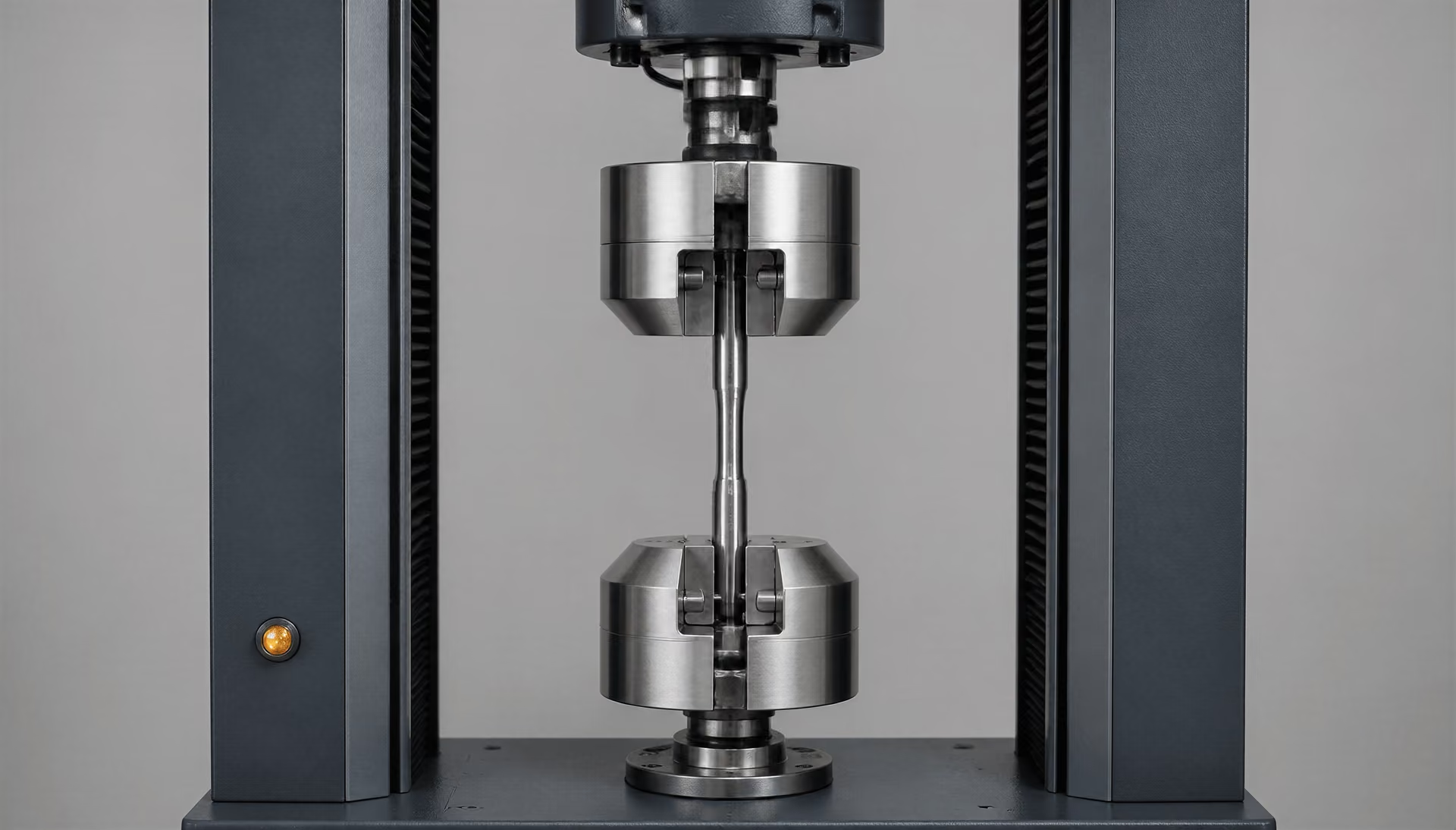
The stress–life, or S–N, method is based on testing specimens under repeated loading until they fracture or reach a specified run-out condition. In the conventional experiment, a machine applies constant-amplitude, force-controlled axial loading. Several specimens are tested at different stress levels, and each result supplies one point relating applied stress to cycles to failure.
For a cyclic stress varying between maximum stress and minimum stress , the stress range is
The stress amplitude is half the range:
The mean stress is
and the stress ratio is
| Quantity | Definition | What it describes |
|---|---|---|
| Stress range, Δσ | σmax − σmin | Total variation between cycle limits |
| Stress amplitude, σa | Δσ/2 | Half the stress range |
| Mean stress, σm | (σmax + σmin)/2 | Average stress level in the cycle |
| Stress ratio, R | σmin/σmax | Relationship between minimum and maximum stress |
These quantities describe different features of the same cycle. A test at has fully reversed stress, with equal tensile and compressive peaks and a zero mean stress. A positive stress ratio indicates that both limits may remain tensile. Two tests with the same stress range can produce different lives when their mean stresses, and therefore their stress ratios, differ.
A common fitted relationship is the Basquin-type power law,
or, when stress range is used,
where or is a fitted constant and is normally negative. Taking logarithms gives a straight-line relation:
The equation is a model of the measured range, not a physical law valid for every steel condition. Its fitted coefficients change with grade, heat treatment, specimen geometry, stress ratio, surface finish, and the selected failure criterion. The 2024 review Fatigue Life Assessment of Steel Structure, A State-Of-The-Art-Review identifies this stress–life representation as the usual power-law form, while also distinguishing fatigue strength, fatigue life, crack initiation, and crack propagation. An S–N test generally records the life to the stated failure condition; it does not automatically separate the cycles spent initiating a crack from those spent growing it.
A smooth, unnotched specimen can therefore provide a material baseline without representing a structure. A machined notch raises local stress, and a welded attachment introduces a weld toe, weld root, residual stress, local geometry, and possible defects. Corrosion, scale, roughness, specimen size, temperature, and loading type can also alter the result. Plain-steel, welded-joint, and welded-attachment details require their own fatigue data or justified corrections.
Logarithmic axes, stress range, and cycles to failure
A conventional S–N plot places stress or stress range on one logarithmic axis and cycles to failure on the other. The Federal Highway Administration describes steel fatigue resistance using curves that plot stress range against cycles to failure on logarithmic axes. Equal distances on either axis represent equal ratios, not equal numerical increments. A horizontal movement from to cycles occupies the same visual distance as a movement from to cycles.
This scaling is necessary because fatigue lives commonly span many orders of magnitude, while stress levels may change by a comparatively modest amount. A downward-sloping line means that a small reduction in cyclic stress can correspond to a large increase in life. The plotted symbol must still be read with its definition: a curve based on cannot be compared directly with one based on unless the factor of two and the stress-ratio conditions are accounted for.
Some steels display an approximately horizontal S–N asymptote at long lives. The 2019 review The gigacycle fatigue strength of steels: a review of structural and operating factors reports that this behavior is common in low-strength steels, whereas high-strength steels may show a second decline beyond approximately cycles. Consequently, assigning a single endurance limit to every steel grade is unsafe. The apparent limit may reflect the tested life range, internal inclusions, surface condition, or the test’s statistical resolution.
Run-out A test result in which a specimen survives to the planned number of cycles without meeting the defined failure criterion. Run-outs are censored observations rather than proof of infinite fatigue life.
A result marked as a run-out means that the specimen did not meet the test’s failure criterion by the designated number of cycles. It is not proof that fracture could never occur. Run-outs are censored observations and affect curve fitting, particularly when many specimens survive the planned test duration. Replication matters because nominally identical specimens fail at different lives. A mean trend, a scatter band, and a design lower bound answer different questions.
Welded-detail design S–N curves may be positioned two standard deviations below the logarithmic mean fatigue-life data, corresponding to approximately 97.5% survival under the stated assumptions. Strong evidence
For welded steel details, the AISC Manual for Repair and Retrofit of Fatigue Cracks in Steel Bridges states that design S–N curves are placed two standard deviations below the logarithmic mean fatigue-life data, corresponding to approximately 97.5% survival under the stated statistical assumptions. That lower-bound curve is a design convention for a detail category, not a universal property of the parent plate.
ISO 1099:2017 and ASTM E466-21 test conditions[2] ISO 1099:2017: Metallic materials — Fatigue testing — Axial force-controlled method. International Organization for Standardization. 2017.
ISO 1099:2017 specifies ambient-temperature, constant-amplitude, axial force-controlled fatigue testing of metallic specimens to obtain relationships between applied stress and cycles to failure at specified stress ratios. The standard defines the testing framework; the resulting curve remains tied to the specimen and conditions used. “Ambient temperature” does not mean that temperature is irrelevant. A reported test should identify the actual test environment and any meaningful temperature variation.
ASTM E466-21 covers force-controlled, constant-amplitude axial fatigue tests on unnotched and notched metallic specimens in air at room temperature. It therefore permits comparison of different specimen forms, but a notched result should not be treated as interchangeable with an unnotched material curve. Notch geometry changes the local stress field and may alter crack initiation.
Neither standard turns a test into a component qualification by itself. Correct alignment is essential because bending superimposed on axial force can change the local stress and invalidate the intended loading condition. The loading frequency must be reported and controlled because heating, environmental interaction, machine dynamics, and rate-sensitive effects can influence life; no single frequency should be assumed from the existence of the standard. Specimen dimensions, machining direction, surface finish, gripping, grade and processing history, stress ratio, and failure definition also belong to the result.
For service assessment, engineers select a curve matching the relevant plain or welded detail and convert the applied loading spectrum into stress cycles. The Steel Construction Institute’s 2018 NSC Technical Digest describes cumulative damage assessment in which damage is summed linearly for a specified detail. That calculation is meaningful only when nominal or local stress definitions, detail geometry, cycle counts, and the S–N curve share compatible assumptions. A laboratory curve is evidence. It is not, by itself, permission to ignore the attachment, notch, weld, surface, or spectrum in the structure.
Why Steel Grade Alone Does Not Predict Fatigue Life
A steel grade identifies a specified range of composition, strength, and production requirements; it does not identify one fatigue performance under every service condition. ASTM A36, ASTM A572 Grade 50, and ASTM A514, for example, differ substantially in yield and tensile strength, but their fatigue lives cannot be ranked from tensile strength alone. Fatigue failure is governed by cyclic stress at a local feature, crack initiation, and crack propagation. Those features may be controlled more by a weld toe, machining mark, inclusion, or corrosion pit than by the parent metal’s nominal strength.
A material S–N curve is therefore baseline evidence for a defined specimen, processing route, geometry, loading mode, stress ratio, and environment. It is not a universal substitution for component testing or design-detail data.
Strength level, microstructure, and the gigacycle regime
Increasing yield strength can raise fatigue strength in smooth, polished specimens, particularly where crack initiation controls failure. The improvement is not proportional, however. Heat treatment changes grain size, martensite or bainite content, carbide distribution, hardness gradients, and inclusion sensitivity. Two heats meeting the same grade designation can consequently produce different scatter in fatigue results. Cold work may increase surface hardness while leaving tensile residual stress or lowering ductility at a critical location.
At long lives, the usual assumption becomes especially unreliable. The 2019 review The gigacycle fatigue strength of steels: a review of structural and operating factors reports that low-strength steels commonly develop an approximately horizontal S–N asymptote. In that range, additional cycles do not require a steadily lower stress in the simple way suggested by an uninterrupted Basquin power law. High-strength steels can behave differently: the review describes a possible second decline in the S–N curve beyond approximately cycles. Internal crack initiation at non-metallic inclusions, often beneath the surface, is one explanation for this very-high-cycle response.
This distinction matters for rotating machinery, springs, rail components, and other parts expected to survive hundreds of millions or billions of cycles. A test stopped at or cycles may miss a later failure mechanism. Conversely, a horizontal “endurance limit” inferred from one dataset should not be transferred to another steel, surface condition, or inclusion population.
ISO 1099:2017 specifies ambient-temperature, constant-amplitude, axial force-controlled fatigue testing at selected stress ratios. ASTM E466-21 covers force-controlled, constant-amplitude axial testing of unnotched and notched metallic specimens in air at room temperature. These conditions define what the resulting curve means. They do not reproduce every service load. Stress ratio, tension–compression versus bending or torsion, mean stress, load sequence, and variable-amplitude damage can all shift the measured relationship.
Notches, size effects, and local stress concentration
Nominal stress is often the wrong stress for predicting crack initiation. At a hole, keyway, thread root, weld toe, sharp fillet, or machining groove, elastic stress concentration raises the local alternating stress above the section-average value. If plasticity develops, the local strain history rather than the elastic nominal stress may control life. A high-strength grade can then lose much of its smooth-specimen advantage because its notch sensitivity and reduced ductility make a small defect more consequential.
A component’s size also changes the result. A larger volume samples more inclusions and contains more potential crack-initiation sites; a larger surface presents more area for scratches, pits, and incomplete fusion. Stress gradients may be less favorable in a large part, and the highly stressed volume can be much greater than that of a laboratory specimen. These are statistical and mechanical size effects, not merely dimensional scaling.
The distinction between plain steel and a structural detail is explicit in design practice. The Federal Highway Administration describes steel fatigue resistance with S–N curves plotting stress range against cycles to failure on logarithmic axes. The Steel Construction Institute’s 2018 NSC Technical Digest describes curves developed for specific plain-steel, welded-joint, and welded-attachment details, with cumulative damage assessed for the relevant detail. For welded steel, the AISC bridge-fatigue manual places design S–N curves two standard deviations below the logarithmic mean fatigue-life data, corresponding to approximately 97.5% survival. That statistical lower bound is not a property of the steel plate alone. It includes the quality and geometry of the detail represented by the test data.
A smooth ASTM specimen cannot therefore stand in for a welded bridge attachment without qualification. The weld toe radius, undercut, residual stress, distortion, weld profile, and possible lack of fusion define a different fatigue problem.
Surface finish, residual stress, temperature, and environment
Surface condition frequently controls the first stage of fatigue. Polishing can remove machining grooves and lower the effective notch severity; turning, grinding burns, scale, and rough milling can leave directional marks that act as crack starters. Shot peening or other surface treatment may introduce compressive residual stress and delay crack initiation. Welding, straightening, machining, and press fitting can instead create tensile residual stress, which reduces the benefit of a favorable nominal mean stress. Residual stress can also relax during cyclic loading or at elevated temperature, so its effect cannot be assigned as a permanent grade correction.
Temperature changes strength, ductility, oxidation, and crack-growth behavior. At low temperature, reduced toughness can make a crack less tolerant of a defect. At high temperature, creep interaction, softening, oxidation, and thermal cycling can reshape the S–N response. Corrosion is more damaging still: a pit supplies a local notch, while corrosion-fatigue repeatedly exposes a fresh crack tip to the environment. Paint, cathodic protection, drainage, and chloride exposure can alter life without changing the steel designation.
Loading type and spectrum complete the problem. Constant-amplitude axial data do not directly describe bending, torsion, contact loading, thermal stress, or a sequence of overloads and small cycles. Design assessments may use detail-specific S–N curves with linear cumulative damage calculations, but the selected curve, stress range, stress ratio treatment, and cycle histogram must correspond to the actual component. Grade strength is one input. Geometry, processing, surface state, environment, and statistical design basis often determine the result.
Welded Steel Details Require Their Own Fatigue Curves

Weld toes, roots, attachments, and geometric discontinuities
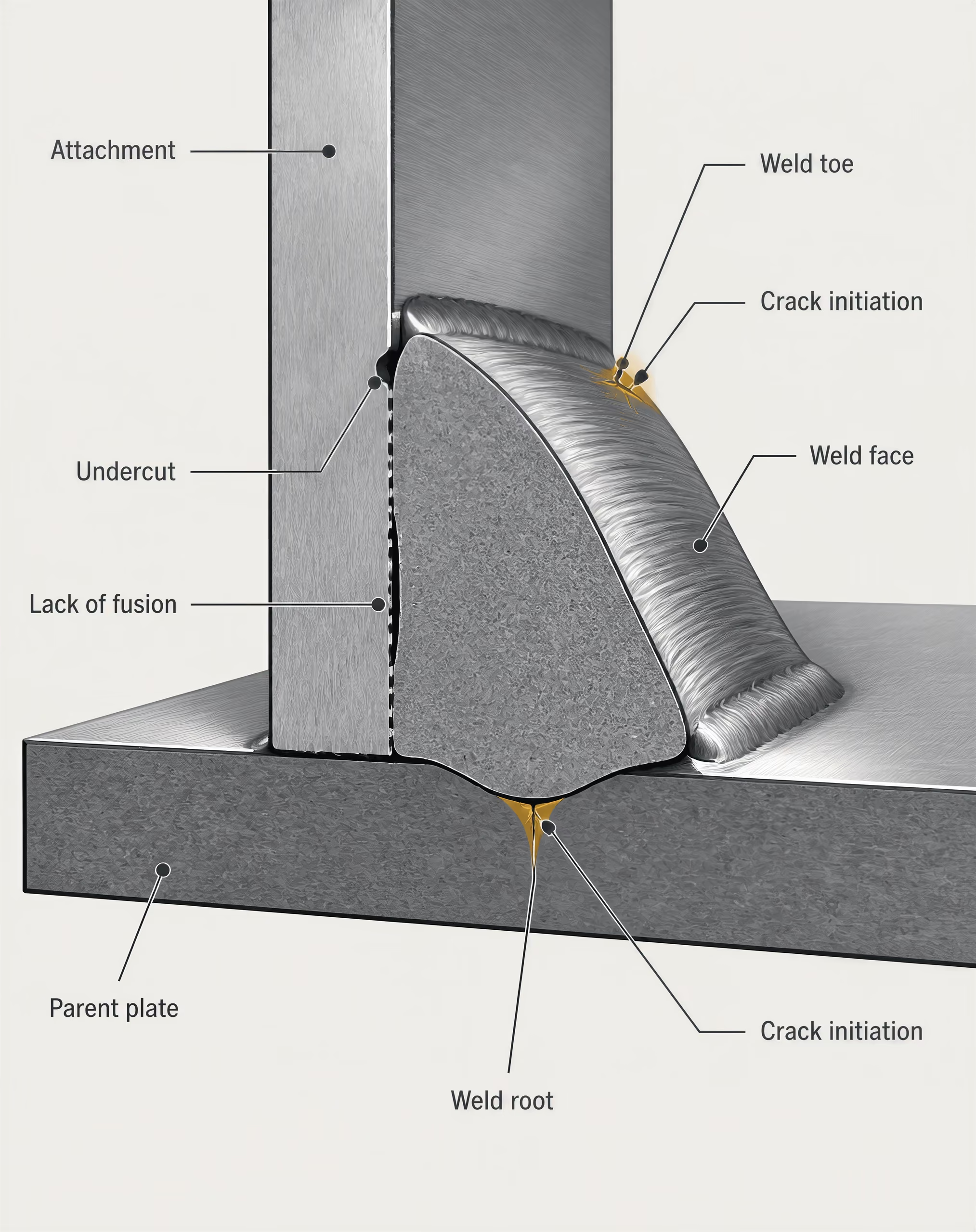
A welded connection does not behave like a polished coupon cut from the parent plate. Its fatigue resistance is governed by the complete detail: weld geometry, toe radius, root profile, attachment shape, plate thickness, alignment, residual stress, distortion, and any crack-like imperfection left by fabrication or service. The steel grade still matters, but it is only one part of the failure mechanism.
At a weld toe, the weld face meets the parent plate at a geometric transition. A small toe radius, excessive convexity, undercut, overlap, or abrupt termination raises the local stress. The weld root can be more severe. Lack of root penetration, lack of fusion, porosity, slag inclusions, and an unfavourable root notch provide short crack-like features before service loading begins. Fatigue cracks usually initiate at, or close to, these locations rather than in an undisturbed region of the plate.
Attachments create additional stress concentrations. A transverse stiffener welded to a girder flange interrupts the force flow through the flange, while a rib-to-deck weld in an orthotropic bridge deck transfers load through a small weld line subject to wheel-induced stress cycles. Longitudinal attachments, gusset plates, brackets, cover plates, and welded repairs each produce their own combination of membrane stress, bending stress, and secondary deformation. Distortion from welding can also leave residual bending and misalignment, so the nominal design geometry may not describe the actual stress field.
Residual tensile stress affects crack growth and the effective stress ratio at the crack tip. In a heavily restrained joint, welding can leave tensile residual stress near the yield strength of the material. This does not mean that every welded detail has the same fatigue strength regardless of applied mean stress, but it does explain why the beneficial effect of a compressive nominal mean stress is often smaller for welded joints than for polished, unwelded specimens. Surface corrosion, fretting, impact damage, and a previous fatigue repair can reduce resistance further.
The parent grade therefore cannot be used as a substitute for the detail. A welded joint made from ASTM A36 steel, ASTM A572/A572M Grade 50 steel, or ASTM A709/A709M Grade 50 steel may fall into a similar fatigue category when the weld configuration and failure location are the controlling features. Increasing yield strength does not proportionally increase the fatigue strength of a weld toe containing the same notch and fabrication imperfection.
Nominal stress, hot-spot stress, and local stress
An S–N curve is meaningful only when its stress definition matches the definition used to derive it. The Federal Highway Administration describes steel fatigue resistance with curves that plot stress range against cycles to failure on logarithmic axes. In a stress–life formulation, often represented by a Basquin-type power law, the selected stress range is related to the number of cycles required to reach the stated failure criterion.
Nominal stress is the average axial, bending, or shear stress calculated away from the discontinuity. It is convenient for a prismatic plate or a classified welded detail whose test data were reported using that same quantity. A nominal-stress curve must not be paired casually with a finite-element peak at the weld toe; those two values include different physical effects.
Stress definitions used for welded details
- Nominal stress
- Average axial, bending, or shear stress calculated away from the discontinuity.
- Hot-spot stress
- Structural stress estimated near the weld toe while excluding the very local notch effect of the weld profile.
- Local stress
- Stress that includes the notch effect at the weld toe or root and requires a defined finite reference stress or notch radius.
Hot-spot stress, also called structural stress in many procedures, estimates the stress at the weld toe by extrapolating stresses from points a short distance away from the sharp notch. It captures the structural stress concentration caused by the attachment and plate geometry while excluding the very local notch effect of the weld profile. This approach is useful when the exact toe radius varies between specimens or cannot be represented reliably in a shell model.
Local stress includes the notch effect at the toe or root. It may be obtained from a refined solid finite-element model, a notch-stress method, or a measured weld profile. Because the theoretical peak at a perfectly sharp geometric corner can be singular, the analyst must define a finite reference stress or notch radius. Local-stress S–N data are not interchangeable with nominal-stress or hot-spot-stress data.
The distinction is practical. A smooth axial coupon tested under ISO 1099:2017 conditions has a uniform force-controlled stress field. ASTM E466-21 covers constant-amplitude axial loading of unnotched and notched metallic specimens in air at room temperature. Neither standard makes a plain specimen equivalent to a welded bridge attachment. Stress ratio, loading type, surface finish, size, temperature, and specimen processing all affect the result.
Detail classification and the limits of parent-metal data
Fatigue design consequently uses detail-specific curves. The Steel Construction Institute’s NSC Technical Digest states that steel-structure damage is assessed with S–N curves developed for particular plain-steel, welded-joint, or welded-attachment details, with cycle damage summed linearly for the selected detail under a given spectrum. A curve for a plain plate is not a permission slip to use the same allowable stress range for a rib-to-deck weld, stiffener termination, bolted connection, or repaired bridge detail.
Design classifications group details with comparable crack-initiation behaviour and specify the stress quantity to which the curve applies. The governing category may be set by a transverse butt weld, weld toe, weld root, attachment end, cope, flange connection, or other feature. FHWA bridge guidance and AISC fatigue provisions use this detail-based approach rather than assigning one universal endurance limit to a steel grade.
The statistical basis matters as much as the geometry. The AISC Manual for Repair and Retrofit of Fatigue Cracks in Steel Bridges describes welded-detail design S–N curves as lower-bound curves placed two standard deviations below the logarithmic mean fatigue-life data, corresponding to approximately 97.5% survival when the stated statistical assumptions apply. That curve is a design boundary, not the average performance of every specimen.
Plain-steel data can establish a material baseline, but transfer requires a defensible stress concentration and correction method. A smooth, polished specimen may initiate a crack only after many cycles of local slip, whereas a weld toe can start with an undercut or incomplete fusion. A corrosion-damaged plate has a different surface condition; a repaired bridge detail may contain residual distortion and a new weld end; a variable-amplitude traffic spectrum introduces sequence effects and occasional overloads absent from constant-amplitude testing.
The claimed endurance limit also requires care. The 2019 review The Gigacycle Fatigue Strength of Steels: A Review of Structural and Operating Factors reports that low-strength steels often show an approximately horizontal S–N asymptote, while high-strength steels can exhibit a second decline beyond about cycles. A welded detail may not display the parent steel’s apparent plateau because weld defects, residual stress, corrosion, and repeated crack growth control the result. The correct curve is therefore the one matched to the welded geometry, stress definition, loading spectrum, and required reliability—not the highest curve available for the plate grade.
Statistical Design Curves and Survival Basis
Scatter in fatigue data
Fatigue life is scattered even when the nominal steel grade, specimen geometry, surface finish, and loading history are closely controlled. Two specimens that appear identical can fail after substantially different numbers of cycles. Small differences in inclusions, grain structure, machining marks, residual stress, alignment, or crack-initiation sites can shift the result. At a component level, weld profile, undercut, porosity, fit-up, attachment stiffness, corrosion, and inspection history add further variation.
An S–N curve therefore describes a population of results, not a precise life prediction for one part. The stress–life method relates stress or stress range to cycles to failure, often with a Basquin-type power law. The Federal Highway Administration describes steel fatigue resistance using stress range plotted against cycles to failure on logarithmic axes. That presentation is useful because fatigue lives may span several orders of magnitude, but it does not remove the underlying scatter.
The test definition matters. ISO 1099:2017 specifies ambient-temperature, constant-amplitude, axial force-controlled testing at stated stress ratios. ASTM E466-21 covers force-controlled, constant-amplitude axial testing of unnotched and notched metallic specimens in air at room temperature. Results from either method should not be transferred casually to a variable-amplitude bridge member, a welded attachment, or a component operating at another temperature and stress ratio.
A polished, unnotched specimen can mainly describe the fatigue response of its specified material and test geometry. It does not automatically represent a machined notch, a bolted connection, a welded diaphragm, or a corrosion-damaged flange. For this reason, design practice uses detail-specific curves for plain steel, welded joints, and welded attachments. The Steel Construction Institute’s 2018 NSC Technical Digest describes fatigue assessment by selecting an S–N curve for the relevant detail and summing damage linearly over the applied stress spectrum.
Lower-bound curves and approximately 97.5% survival
For welded steel details, the AISC Manual for Repair and Retrofit of Fatigue Cracks in Steel Bridges (2013) describes design S–N curves as lower-bound curves placed two standard deviations below the logarithmic mean fatigue-life data. Under the statistical assumptions used for that data set, this corresponds to approximately 97.5% survival. The logarithmic scale is important: the standard deviations apply to log cycles to failure, not directly to cycles on an arithmetic scale.
This convention supplies a practical margin between observed average behavior and the curve used for design. It is not a guarantee that 97.5% of every manufactured component will survive the stated number of cycles. The percentage applies to the tested detail family, its test conditions, its statistical model, and the assumed failure definition. A weld with a different profile, residual-stress state, inspection quality, corrosion exposure, or load spectrum may not belong to that same population.
Nor does the lower-bound curve mean that failures below it are impossible. Statistical tails remain, and model error can be as important as specimen scatter. The curve also concerns the selected fatigue criterion—often crack initiation or complete failure as defined by the test—not necessarily serviceability, detectable cracking, leak tightness, or residual load capacity.
Mean curves, design curves, and uncertainty
| Curve or limit | Primary question answered | Interpretation |
|---|---|---|
| Mean regression line | What is the average logarithmic life? | Central tendency of the matching test population |
| Lower-bound design curve | What conservative design boundary is selected? | A prescribed statistical allowance below the mean curve |
| Confidence limit | How uncertain is the estimated mean? | Uncertainty caused by the finite test sample |
| Prediction limit | Where may an individual future result fall? | Includes population scatter and fitted-mean uncertainty |
A mean regression line estimates the average logarithmic fatigue life at each stress range. Roughly half of a matching population would be expected to fail before that line and half after it, although the exact interpretation depends on the fitted distribution and censoring of run-outs. It is an estimate of central tendency, not a safe design boundary.
A lower-bound design curve shifts the fitted relation downward by a prescribed statistical allowance, such as the two-standard-deviation AISC basis. A confidence limit answers a different question: how uncertain is the estimated mean curve because only a finite number of tests were performed? A prediction limit addresses where an individual future result, or a specified fraction of future results, may fall. Confidence limits concern the fitted population mean; prediction limits include specimen-to-specimen scatter as well as uncertainty in the fitted mean.
Those distinctions matter when comparing published curves. A narrow confidence band around a mean does not imply narrow component scatter. Conversely, a conservative design curve may incorporate a survival fraction without covering errors caused by choosing the wrong weld category or stress definition. Nominal stress, local notch stress, stress range, and stress ratio must match the curve’s basis.
The curve’s long-life shape also requires judgment. A 2019 review of gigacycle fatigue reports that low-strength steels commonly approach a near-horizontal S–N asymptote, while high-strength steels may show a second decline beyond about cycles. Treating every apparent plateau as a universal endurance limit can therefore be unsafe. A stated survival basis is meaningful only when the material, detail, loading spectrum, environment, and statistical population remain comparable.
From Constant-Amplitude Testing to Service-Life Assessment
Laboratory S–N data normally come from constant-amplitude tests, not from the irregular loading histories found in service. ISO 1099:2017 specifies ambient-temperature, axial, force-controlled fatigue tests at constant amplitude and selected stress ratios. ASTM E466-21 similarly covers unnotched and notched metallic specimens subjected to constant-amplitude axial loading in air at room temperature. These methods are valuable because they isolate the relation between applied stress and cycles to failure, but that isolation is also a limitation.
The stress–life method expresses fatigue behaviour as stress, or stress range, against cycles to failure. A Basquin-type relation is often fitted on logarithmic axes, while the Federal Highway Administration describes steel fatigue resistance through S–N curves plotting stress range against cycles to failure. Such a curve belongs to the test conditions that produced it. Specimen geometry, surface finish, material processing, stress ratio, loading type, temperature and failure definition all matter.
A polished, smooth specimen made from a plate of S275JR steel cannot be transferred directly to a welded bridge attachment. The attachment contains a weld toe or root, local geometric discontinuities and residual stresses; the relevant design curve is therefore a welded-detail curve, not simply the parent-metal curve. A machined notch, a corroded crane girder and a pressure-vessel nozzle each require their own treatment. The distinction is important: fatigue strength describes resistance at a specified life, fatigue life describes the cycles associated with a specified stress condition, and neither quantity alone describes crack propagation after a crack has formed.
Variable-amplitude loading and cycle counting
Bridges experience different stress ranges as vehicles cross at different speeds and weights. Crane structures see starts, stops, lifts and trolley movements. Vehicles encounter acceleration, braking, road irregularities and changes in payload. Pressure equipment may cycle between operating states, while rotating machinery combines start-up transients with long periods of steady operation. The resulting stress history changes in both range and mean stress.
Rainflow counting A cycle-counting method that converts an irregular stress-time history into closed and half cycles with associated stress ranges, enabling variable-amplitude fatigue calculations.
A service record or calculated load model is therefore converted into a stress spectrum. One practical approach divides the spectrum into blocks: for example, a number of cycles at a high stress range, a larger number at an intermediate range, and many cycles at a low range. Rainflow counting is commonly used to reduce a measured or simulated stress-time history to closed and half cycles, each assigned a stress range and usually a mean stress or stress ratio. The counted cycles must then be related to the correct structural response: nominal stress for a classified weld detail, hot-spot stress for an appropriate welded geometry, or local notch stress where the method and data support it.
The stress ratio, , can affect fatigue life, especially in unwelded material. Mean-stress corrections may be needed when test data and service conditions have different values of . Welded-detail classifications often incorporate residual-stress assumptions and are not interchangeable with polished-specimen data. Applying a correction twice, or applying one outside its validated range, can produce a misleading life estimate.
Linear cumulative damage for fatigue details
For each stress-range block, the assessor selects the S–N relation for the actual detail: plain steel, a bolted connection, a weld category, a welded attachment or another classified feature. If cycles occur at stress range , and is the cycles to failure predicted by that relation, the damage fraction is . The linear cumulative-damage rule then gives
The Steel Construction Institute’s NSC Technical Digest (2018) states that cumulative damage is summed linearly for a given fatigue detail. In the simplest assessment, failure is associated with reaching unity. This is an engineering framework, not a universal law of steel. It assumes that damage fractions from different stress levels can be added without accounting explicitly for load-sequence effects, interaction between cracks, changing residual stress or evolving stiffness.
Those assumptions may be acceptable when the detail category, spectrum and analysis method match the evidence behind the design curve. For welded steel details, the AISC bridge-fatigue manual describes design S–N curves as lower-bound curves placed two standard deviations below the logarithmic mean fatigue-life data, corresponding to approximately 97.5% survival. That statistical basis is different from claiming that every specimen, component or service history will reach the same limiting damage value.
A service-life calculation should also state whether failure means visible crack initiation, a through-thickness crack, loss of section, or a defined fracture limit. Low-strength steels often show an approximately horizontal S–N asymptote, but the 2019 review The gigacycle fatigue strength of steels: a review of structural and operating factors reports that high-strength steels can show a second decline beyond about cycles. A conventional endurance-limit assumption may therefore be unsafe for very high-cycle machinery.

When S–N analysis is insufficient
S–N analysis is primarily a crack-initiation or total-life design method calibrated against a specified detail. It becomes insufficient when a crack is already known or when inspection has revealed a flaw whose size and location can be measured. At that point, the central question changes from “How many cycles precede failure in an uncracked detail?” to “How will this crack grow under the future spectrum, and when will it reach a critical size?”
Fracture-mechanics or crack-growth analysis is required for known cracks, inspection findings, severe corrosion and repairs with uncertain remaining section. Such analyses can use stress-intensity factors, crack-growth laws and crack-closure assumptions to calculate progression between inspections. Residual stress is especially significant around welds and may alter crack-growth behaviour even when the nominal service stress appears modest.
An S–N curve may also be inadequate under complex multiaxial loading, substantial plasticity, pronounced local notch effects, thermal cycling or load histories containing severe overloads. Very high-cycle service is another warning sign because internal inclusions, persistent slip bands and subsurface crack initiation can govern behaviour beyond the range represented by ordinary tests. In these cases, the assessment should identify the controlling failure mechanism rather than force every stress history into a single material curve.
A Practical Reading Guide for Steel Fatigue Data
Questions to ask before using an S–N curve
An S–N curve is not a universal property of “steel.” It describes a defined experiment or design population: stress (or stress range) on one axis and cycles to failure on the other, usually with both axes logarithmic. The Federal Highway Administration describes this format for steel fatigue resistance, while the stress–life method commonly fits the data with a Basquin-type power law.
First identify what was tested. ASTM A36, ASTM A572 Grade 50, and EN 10025-2 S355 may have different yield strengths, inclusions, heat treatments, and processing histories, but grade designation alone still does not define fatigue performance. Plate thickness, rolling direction, normalized condition, quench-and-temper treatment, residual stress, and weld thermal history can change the result. Ask whether the curve represents plain base metal, a machined notch, a welded joint, or a specified attachment detail.
Then identify the loading definition. ISO 1099:2017 specifies ambient-temperature, constant-amplitude, axial, force-controlled testing at stated stress ratios. ASTM E466-21 covers axial unnotched and notched metallic specimens under constant-amplitude periodic loading in air at room temperature. Neither standard makes its data automatically applicable to bending, torsion, contact loading, thermal cycling, corrosion, or variable-amplitude service.
Stress range, maximum and minimum stress, stress ratio, nominal versus local stress, loading mode, specimen size, surface finish, temperature, and environment all matter. A polished coupon with carefully controlled geometry does not represent a corroded component or a welded bridge attachment unless the transfer assumptions are stated and justified.
Common interpretation errors
The most common mistake is reading a horizontal tail as a guaranteed endurance limit. A short test may simply have stopped before a later decline became visible. The 2019 review The Gigacycle Fatigue Strength of Steels: A Review of Structural and Operating Factors reports that low-strength steels often show an approximately horizontal S–N asymptote, whereas high-strength steels can exhibit a second fall beyond about 10^7 cycles.
Curves also become misleading when their stress definitions differ. One may use nominal stress range; another may use hot-spot stress, notch-root stress, or structural stress. Their positions cannot be compared directly. Nor should polished base-metal data be transferred to welded details. Weld toe geometry, undercut, porosity, residual tensile stress, and repair quality often control the result more strongly than the parent steel grade.
A design lower bound is not a direct material property. For welded details, the AISC bridge-fatigue manual describes curves placed two standard deviations below the logarithmic mean fatigue-life data, corresponding to approximately 97.5% survival. That curve includes statistical protection and detail effects. It is not the intrinsic fatigue strength of the steel itself.
Finally, constant-amplitude life cannot be assumed for service containing overloads, changing amplitudes, or load-sequence effects. The Steel Construction Institute’s NSC Technical Digest treats damage by detail-specific S–N curves and linear cumulative damage assessment; the selected spectrum remains part of the calculation.
Minimum reporting checklist
Minimum S–N data checklist
- Material Steel designation, product form, thickness, heat treatment, and processing condition.
- Detail Whether the curve applies to plain material, a notch, a weld, or a defined attachment detail.
- Loading Stress range, stress ratio, stress definition, loading mode, temperature, and environment.
- Surface and fabrication Surface condition, weld geometry and quality, specimen scale, and failure criterion.
- Statistics Sample count, run-outs, scatter model, confidence or survival basis, and design adjustments.
- Service spectrum Whether loading is constant or variable amplitude and how cumulative damage is assessed.
Before using a curve, record:
- steel designation, product form, thickness, heat treatment, and processing condition;
- whether it applies to plain material, a notch, a weld, or a defined attachment detail;
- stress range and stress ratio, plus nominal, local, hot-spot, or structural stress definition;
- axial, bending, torsional, or mixed loading; temperature and environment;
- surface condition, weld geometry and quality, specimen scale, and failure criterion;
- whether failure means crack initiation, detectable crack growth, or final fracture;
- sample count, run-outs, scatter model, confidence or survival basis, and design adjustments;
- whether the service spectrum is constant amplitude or variable amplitude, and how cumulative damage is assessed.
References
- [1] ASTM E466-21: Standard Practice for Conducting Force Controlled Constant Amplitude Axial Fatigue Tests of Metallic Materials. 2021. https://store.astm.org/e0466-21.html
- [2] ISO 1099:2017: Metallic materials — Fatigue testing — Axial force-controlled method. 2017. https://www.iso.org/standard/67847.html