




What Steel Elastic Constants Mean—and What They Do Not Mean
Elastic constants are parameters that connect applied stress with the resulting strain while a material remains within its elastic range. In that range, removing the load allows the specimen to return, at least approximately, to its original dimensions. For a simple tensile test, Young’s modulus is the ratio of axial stress to axial strain,
This relation describes the slope of the initial, recoverable part of a stress–strain curve. It does not describe the entire curve, and it does not state how much stress the steel can withstand before permanent deformation or fracture.
The six related isotropic quantities
- Young’s modulus E
- Axial stiffness in tension or compression.
- Poisson’s ratio ν
- The ratio of transverse strain to axial strain under elastic loading.
- Bulk modulus K or B
- Resistance to uniform volumetric compression.
- Shear modulus G
- Resistance to angular distortion under shear.
- Lamé’s first parameter λ
- A parameter in the isotropic stress–strain constitutive law.
- 2μ
- Twice the second Lamé parameter, where μ equals G.
Only two elastic constants are independent for an isotropic, linear-elastic solid. Strong evidence
For an isotropic, linear-elastic solid, only two elastic constants are independent. A commonly used set contains Young’s modulus , Poisson’s ratio , bulk modulus or , shear modulus , Lamé’s first parameter , and , where . Sandia National Laboratories lists these six related quantities and states that and determine the others. For example,
and
Bulk modulus A measure of resistance to uniform volume change under pressure; it is commonly written K or B.
The notation varies: NIST and other sources often use for bulk modulus, while engineering texts and finite-element software often use . They describe the same isotropic property.
Elastic response versus strength and plasticity
| Property | Primary response | What it does not measure |
|---|---|---|
| Young’s modulus E | Axial elastic strain | Yield strength or fracture strength |
| Shear modulus G | Angular distortion under shear | Shear yield strength |
| Bulk modulus K or B | Uniform volume change under pressure | Tensile ductility |
| Hardness | Resistance to localized indentation | Elastic stiffness |
| Toughness | Energy absorption and crack resistance | Initial stress–strain slope |
Elasticity answers a narrow question: how much strain accompanies a given stress before permanent deformation begins? Strength answers different questions. Yield strength identifies the stress associated with the onset of specified plastic strain; tensile strength is the maximum engineering stress reached during a tensile test; fracture strength concerns separation of the specimen. None of these is another name for Young’s modulus.
A steel can have a high yield strength and nearly the same Young’s modulus as a lower-strength steel of similar composition. Cold working, precipitation hardening, or martensitic transformation may greatly increase yield strength and hardness while changing the small-strain tensile modulus far less. The reason is that strengthening mechanisms obstruct dislocation motion, whereas the initial elastic response mainly reflects atomic bond stiffness and the aggregate crystal structure. This distinction is central when comparing, for example, a quenched-and-tempered low-alloy steel with an annealed product of related chemistry.
Plasticity begins when the stress–strain relation no longer follows the original linear elastic slope. A plastic constitutive model then needs information such as yield criteria, hardening law, flow rule, strain-rate sensitivity, and temperature dependence. Young’s modulus alone supplies none of that information. A finite-element model that contains an accurate but an unsuitable yield surface can still predict permanent deformation badly.
Other mechanical properties answer still different questions. Hardness measures resistance to localized indentation and often correlates with strength within a controlled family of steels, but it is not a modulus. Toughness concerns energy absorption and crack resistance under a specified test condition. Fatigue resistance concerns damage accumulation under repeated or fluctuating loading. A steel may have similar elastic modulus to another grade but different hardness, impact toughness, crack-growth behavior, or fatigue life.
Elasticity also does not mean that every loading cycle is perfectly reversible. Real steel can show microplasticity, anelasticity, residual stress effects, hysteresis, or damage before a conventional yield point is obvious. The modulus reported for a particular test is therefore tied to its strain range, loading rate, cycle history, and data-reduction method.
Modulus as stiffness, not failure stress
A modulus measures stiffness: the stress required to produce a specified elastic strain in a defined deformation mode. Young’s modulus concerns axial extension or contraction. The shear modulus describes resistance to shape change under shear stress. The bulk modulus describes resistance to uniform volume change under pressure. OpenStax gives these corresponding physical interpretations for tensile, shear, and volumetric deformation.
A large modulus means that a given stress produces a smaller elastic strain. It does not mean that the material supports a larger stress before yielding or fracture. Consider two steel components with the same but different yield strengths. Under the same service stress, they undergo approximately the same elastic extension. The higher-strength component can tolerate a greater stress before plastic deformation, but it is not appreciably stiffer in the initial elastic response merely because its yield strength is higher.
The bulk modulus has a particularly clear thermodynamic definition. In its 1982 handbook chapter, the National Institute of Standards and Technology writes
[1] Bulk modulus definition. National Institute of Standards and Technology. NIST handbook chapter, 1982.
where is volume, is pressure, and the derivative is taken at constant temperature. This is a volumetric property, not a tensile failure limit. Steel is difficult to compress uniformly, so its bulk modulus is high; that fact says little by itself about tensile ductility or fracture toughness.
Modulus also should not be confused with resilience. The elastic energy stored per unit volume depends on stress and modulus, and the recoverable energy up to yield depends on both modulus and yield strength. Raising yield strength can therefore increase elastic energy capacity even when changes only slightly.
Why a steel grade does not have one universal modulus
| Designation or family | What it identifies | Why the label is insufficient for one modulus |
|---|---|---|
| ASTM A36 | A structural-steel product specification | Product form, direction, temperature, and test method still matter |
| ASTM A572 Grade 50 | A grade within a structural-steel specification | Strength requirements do not define one universal elastic number |
| EN 10025-2 S355JR | A European structural-steel designation | Delivery condition and product details affect reported properties |
| AISI 304 | An austenitic stainless-steel grade | Texture, phase condition, temperature, and method can vary |
| 17-4 PH H900 | A precipitation-hardening stainless-steel condition | Heat-treatment condition is part of the material description |
A designation such as ASTM A36, ASTM A572 Grade 50, EN 10025-2 S355JR, or AISI 304 identifies a specification, composition range, product condition, or required performance set; it does not define one immutable elastic number for every specimen made to that designation. The measured response depends on material state and test conditions.
Temperature is one major variable. Elastic constants generally change with temperature, and phase transformations can produce larger changes when they alter the crystal structure or phase mixture. A National Bureau of Standards report published in 1981 measured the elastic constants of Fe-5Cr-26Mn austenitic steel from 76 to 400 K using longitudinal- and transverse-mode sound velocities. That temperature span alone demonstrates why a value without a test temperature is incomplete.
Quasi-isotropic An effective material response that is close enough to isotropic for a defined calculation, direction range, and scale, even though individual grains remain anisotropic.
Texture and direction matter as well. Individual ferrite, austenite, or martensite crystals are elastically anisotropic, meaning their stiffness depends on crystallographic direction. Rolled plate, forged bar, drawn wire, and additively manufactured material can develop preferred orientations. A polycrystalline aggregate may behave approximately isotropically when crystal orientations are sufficiently distributed, but a strongly textured product may require direction-specific constants. The longitudinal modulus in the rolling direction need not equal the value through the thickness.
Phase constitution, inclusions, porosity, residual stress, grain structure, and product form also influence the measured aggregate response. Weld metal and heat-affected zones can differ from parent plate even when they are covered by the same project specification. Single-crystal constants cannot simply be substituted for polycrystalline design values. The NIST handbook explains how quasi-isotropic Young’s, shear, bulk, and related moduli can be derived from single-crystal elastic-stiffness data for cubic and hexagonal materials, but that calculation depends on crystal symmetry and assumptions about orientation averaging.
| Method | Primary measured response | Typical reported constants | Main qualifications |
|---|---|---|---|
| Tensile test | Force and axial strain | Static or quasi-static E; ν if lateral strain is measured | Sensitive to alignment, extensometer setup, compliance, and slope interval |
| Compression test | Force and axial displacement or strain | Axial modulus | End friction, buckling, and platen alignment can affect the result |
| Sonic resonance | Natural resonant frequencies | Dynamic E, G, and ν | Depends on geometry, density, support conditions, damping, and frequency |
| Ultrasonic wave velocity | Longitudinal and transverse wave speeds | Dynamic G, K, E, and ν | Depends on density, temperature, direction, polarization, and mode identification |
| Hydrostatic compression | Pressure–volume response | Bulk modulus K or B | Requires controlled pressure, volume measurement, and temperature |
ASTM E1875-20a specifies dynamic measurement of Young’s modulus, shear modulus, and Poisson’s ratio by sonic resonance. Strong evidence
Measurement method changes the reported result. A slow tensile test produces a static or secant/tangent modulus based on force and displacement, while ultrasonic or resonance methods determine a dynamic modulus from wave speed or natural frequency. ASTM E1875-20a specifies determination of dynamic Young’s modulus, shear modulus, and Poisson’s ratio “by sonic resonance.” Dynamic values can differ from static values because of frequency, damping, machine compliance, strain amplitude, and the treatment of nonideal portions of the specimen.
Consequently, a useful modulus report states at least the steel designation, product form and condition, temperature, loading direction, deformation mode, and measurement method. It should also identify whether the value is measured, calculated from other constants, or adopted as a design assumption. Engineering ToolBox gives an approximate bulk modulus of 163 GPa for “stainless steel,” but that is a secondary reference estimate, not a universal value for every stainless-steel grade, heat treatment, texture, temperature, or test method. Using one number for every product can be acceptable for a preliminary isotropic calculation when the assumption is declared. Presenting it as a grade-independent material fact is not.
The Two-Constant Basis of Isotropic Linear Elasticity
Linear elasticity describes the reversible part of a material’s response while stress and strain remain sufficiently small for a linear relation to apply. The word isotropic adds a separate condition: the response is assumed to be the same in every direction. Under those two assumptions, the elastic stiffness tensor has far fewer independent terms than a general anisotropic solid. Six commonly reported quantities—Young’s modulus , Poisson’s ratio , bulk modulus or , shear modulus , Lamé’s first parameter , and —can therefore be expressed from only two selected constants.
That result applies to the constitutive model, not automatically to every measured value reported for steel. Temperature, phase constitution, crystallographic texture, porosity, residual stress, specimen orientation, frequency, and the test method can all affect the measured response. A value used in an isotropic finite-element model is often an effective engineering property rather than a complete description of the material’s microstructure.

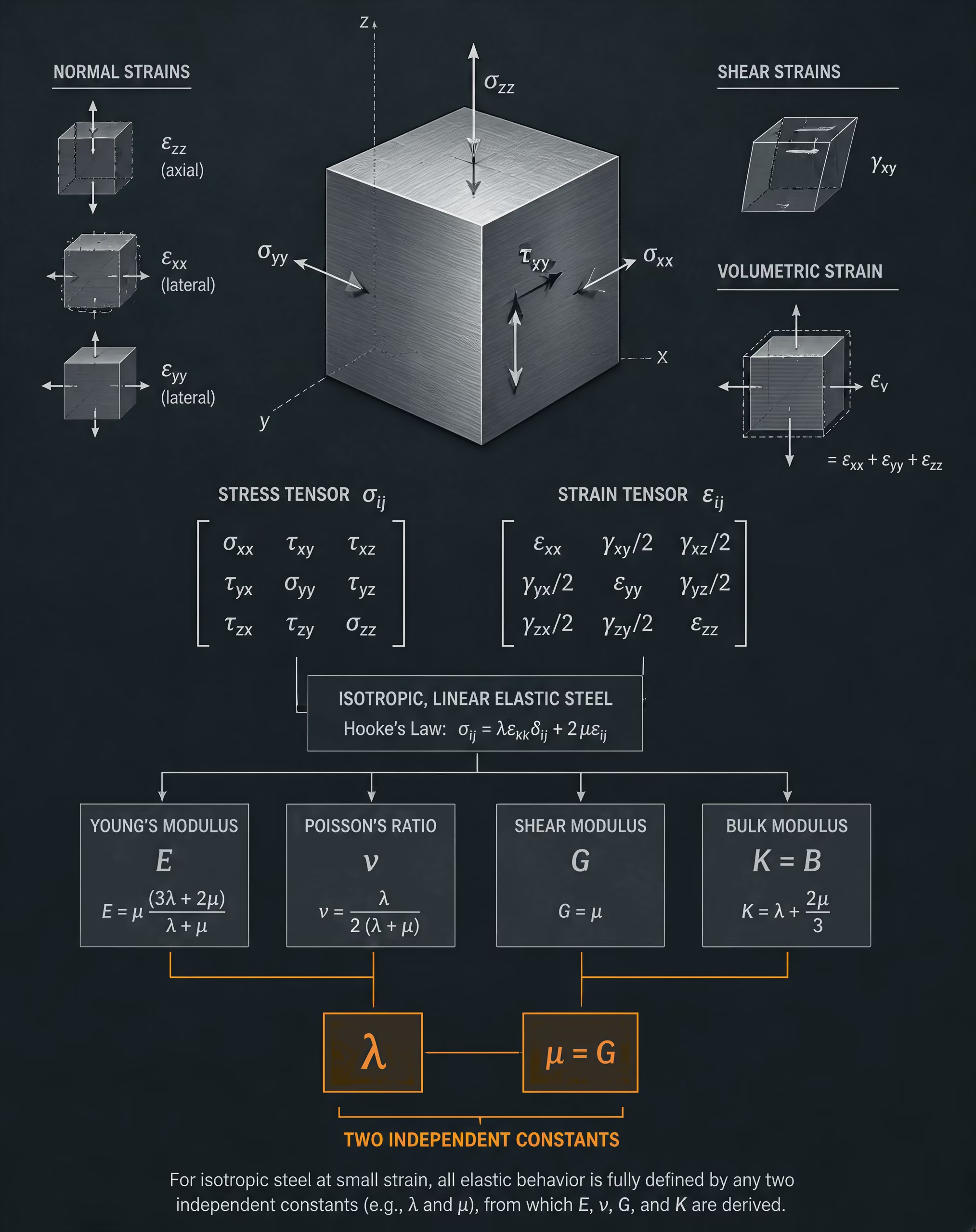
Why only two independent constants are needed
Stress and strain are second-order tensors. In the most general linear elastic solid, the relation between them requires a fourth-order stiffness tensor, with many possible directional couplings. The symmetry of the stress and strain tensors reduces the number of independent terms, and material symmetry reduces it further. Isotropy imposes the strongest ordinary material symmetry: no direction is mechanically distinguished.
The isotropic stress–strain relation can be written as
where is the stress tensor, is the strain tensor, is the Kronecker delta, and and are Lamé parameters. Thus, and form one valid pair of independent constants. The shear modulus is , so using and is equivalent.
Springer’s Elasticity of Solids (2020) states the central result directly: for an isotropic solid, only two elastic constants are independent. Sandia National Laboratories’ Sierra documentation lists the related isotropic set as Young’s modulus , Poisson’s ratio , bulk modulus , shear modulus , Lamé’s first parameter , and , and states that and determine the others. The appearance of six names does not create six separately adjustable material properties.
For the common pair, the conversions are
and
The inverse relations are also useful:
These equations are not empirical correlations limited to one steel family. They follow from the isotropic linear-elastic constitutive law. They also impose consistency requirements. For a stable, ordinary isotropic solid, , , and . As approaches 0.5, the material becomes nearly incompressible in the model: grows much larger than , while remains linked to both.
The physical meanings differ even though the constants are mathematically connected. OpenStax describes Young’s modulus as the ratio governing tensile response, the bulk modulus as the response to volumetric compression, and the shear modulus as the response to shear deformation. A tensile test primarily supplies , but the lateral strain measured beside the axial strain supplies . A pressure-volume experiment targets , while torsion or a shear-wave measurement targets . Once any consistent pair is known, the other moduli are calculated rather than independently selected.
The thermodynamic definition of bulk modulus makes its distinction from Young’s modulus explicit:
This expression, given by the National Institute of Standards and Technology in 1982, describes resistance to volume change under pressure at constant temperature. It does not mean that a tabulated bulk modulus is interchangeable with a tensile modulus. Their numerical relationship exists only after the isotropic constitutive assumptions are applied.
E and ν as a practical input pair
Engineering calculations commonly use and because they map naturally onto a uniaxial tensile test and are directly supported by standard structural-material data. In a three-dimensional isotropic model, entering those two quantities allows the software to construct , , , and without additional material constants. Entering all six can create an inconsistent model if the values do not satisfy the conversion equations.
This is especially important when values come from different sources. A static tensile modulus, a dynamic modulus from resonance, and a bulk-modulus estimate may each be valid for their own measurement conditions while failing to reproduce one another exactly through the isotropic equations. ASTM E1875-20a specifies determination of dynamic Young’s modulus, shear modulus, and Poisson’s ratio “by sonic resonance.” Those are frequency-dependent or rate-sensitive measurements in practice, even when the material remains within its elastic range. They should not be assumed identical to low-rate tensile values without checking the test conditions.
A secondary reference, Engineering ToolBox, gives an approximate bulk modulus of 163 GPa for stainless steel. That number is a reference estimate, not a universal constant for every stainless-steel grade, heat treatment, temperature, product form, or test method. It should not be combined casually with an unrelated or value and then presented as a measured grade-specific property. The same caution applies to values in the ASM Steel Castings Handbook, where modulus of elasticity, Poisson’s ratio, shear modulus, and related physical properties are presented as characteristic data for steel castings. “Steel” is not one fixed elastic specimen.
The distinction between static and dynamic properties matters in design. Dynamic tests infer elastic constants from resonant frequencies or wave speeds; static tests infer them from force, displacement, and strain. A dynamic modulus can differ because of frequency, damping, microstructural mechanisms, temperature, and instrumentation. The National Bureau of Standards report on Fe-5Cr-26Mn austenitic steel measured elastic constants over 76–400 K from longitudinal- and transverse-mode sound velocities. That range demonstrates why a value without temperature and method can be incomplete, even when the material designation is precise.
The role of isotropy and quasi-isotropy
A polycrystalline steel can behave approximately isotropically when its grains are small, numerous, and sufficiently randomized in orientation. The individual crystals remain anisotropic, but directional effects can average out over a representative volume. This is the basis for using one effective and one effective in many structural calculations.
The approximation weakens when processing creates strong texture. Rolling, forging, additive manufacturing, directional solidification, and weld thermal cycles can produce preferred crystallographic orientations. A plate may then have different longitudinal, transverse, and through-thickness properties. A cast product can show another pattern because of dendritic structure, segregation, porosity, and local grain orientation. Phase constitution also matters: ferrite, austenite, martensite, bainite, and retained austenite do not contribute identical single-crystal elastic behavior.
Quasi-isotropic describes an effective response that is close enough to isotropic for a specified purpose, direction range, and scale. It does not erase crystal anisotropy or guarantee that every modulus measured in every orientation will agree. The NIST handbook chapter on monocrystal elastic constants explains how polycrystalline , , , longitudinal modulus, and can be derived from single-crystal stiffness data for cubic and hexagonal elements. That route makes the averaging assumption visible instead of treating the resulting polycrystalline constants as fundamental values.
For a strongly textured steel, an anisotropic elasticity model may require more than two independent constants and must retain specimen orientation. For a quasi-isotropic steel component, two effective constants may be sufficient for the intended calculation, provided the assumption has been checked against measurements. Oxford Academic’s Constitutive Response chapter likewise frames isotropic linear elasticity around two independent constants. The practical question is therefore not whether steel has six independent elastic moduli. It does not under the isotropic model. The question is whether the chosen two constants represent the material, temperature, direction, and measurement regime relevant to the calculation.
Young’s Modulus E in Steel
Young’s modulus, , describes the stiffness of a material in uniaxial tension or compression. Under the applicable linear-elastic definition, it is the ratio of axial stress to axial strain:
Here, is the normal stress acting along the specimen axis and is the corresponding axial strain. For a perfectly linear response, the stress–strain graph is a straight line through the origin, and is its slope. The units are pascals, normally reported for steel in gigapascals.
That definition applies only over the part of loading where the material response is linear and recoverable. It does not mean that every stress-to-strain ratio measured during a steel test is Young’s modulus. Once plastic strain, phase transformation, damage, or substantial nonlinearity appears, the selected slope or ratio describes a different property.
Uniaxial stress and axial strain
A uniaxial tensile test applies a force along one principal direction of a specimen. The engineering axial stress is commonly calculated from the applied force divided by the original cross-sectional area:
Engineering axial strain is the change in gauge length divided by its original length:
At small strain, these definitions provide the usual engineering value of . A test extensometer or strain gauge measures the elongation over a specified gauge length, while the testing machine records force and displacement. The measured slope can be affected by machine compliance, grip movement, specimen alignment, surface condition, and the method used to determine the initial portion of the curve.
In the elastic range, a tensile specimen also contracts laterally. Poisson’s ratio, , relates lateral strain to axial strain, usually as
[3] Elasticity of Solids. Springer Nature. Springer book chapter, 2020.
For an isotropic linear-elastic solid, and determine the other elastic constants. The Sandia Sierra documentation lists the related isotropic set as Young’s modulus , Poisson’s ratio , bulk modulus , shear modulus , Lamé’s first parameter , and ; its statement that and determine the others reflects the two-constant structure of isotropic elasticity. Springer’s Elasticity of Solids likewise states that only two elastic constants are independent for an isotropic solid.
The relationships commonly used in design are
and
where is the shear modulus and , also written , is the bulk modulus. These equations do not make , , , and four independent grade properties. They connect measurements under different deformation modes when the isotropic, linear-elastic assumptions are appropriate.
The distinction between deformation modes matters. Young’s modulus concerns axial extension or contraction, shear modulus concerns angular distortion under shear, and bulk modulus concerns volume change under hydrostatic pressure. OpenStax presents these as separate physical interpretations of elastic response. The NIST handbook’s 1982 treatment defines the bulk modulus thermodynamically as
so its value concerns pressure-driven volume change at specified temperature, not simply the slope of a tensile stress–strain curve.
Steel is often treated as isotropic in ordinary engineering calculations because a polycrystalline product may contain many crystallographic orientations. That approximation can fail in strongly textured sheet, heavily worked bar, rolled plate, weldments, additively manufactured material, or single-crystal research specimens. Cubic ferrite and austenite crystals have direction-dependent elastic stiffnesses even though an aggregate with suitably distributed orientations can appear quasi-isotropic. NIST explains how polycrystalline , , , longitudinal modulus, and Poisson’s ratio can be calculated from single-crystal elastic-stiffness data for cubic and hexagonal materials.
Consequently, a value reported for “steel” is not automatically a universal constant for every product form. Chemical composition, ferrite, pearlite, bainite, martensite, retained austenite, carbide populations, porosity, texture, and residual stress can affect the measured response. The effect may be small in one test configuration and important in another.
Secant, tangent, and initial elastic modulus
The initial elastic modulus is the slope of the stress–strain curve at, or very near, zero stress and strain. In differential form,
provided the curve is sufficiently linear and the measurement system has been corrected. This is the value most closely associated with the textbook definition of Young’s modulus.
A tangent modulus is the local slope at a selected point:
If the curve remains linear, the tangent modulus equals the initial modulus. Near yield, however, steel may show curvature caused by the onset of plasticity, dislocation motion, Lüders strain, transformation effects, or testing artifacts. The tangent modulus then changes with stress and strain. It must be reported with the point or strain interval at which it was measured.
A secant modulus is the slope of a line from a chosen origin to a selected point on the curve:
for that selected point. It averages the response over the interval rather than describing the local slope. If the curve bends away from linearity, the secant and tangent values differ. A secant modulus taken at a stress beyond first yield can be much lower than the initial elastic modulus because the total strain includes plastic strain.
These terms are therefore not interchangeable. Calling a secant value “Young’s modulus” without stating the strain or stress range can mislead a design calculation. The same problem arises when a machine reports a slope from crosshead displacement rather than directly measured gauge strain. Grip seating and frame deformation can distort the early curve, while plasticity can distort a later one.
Prior deformation also matters. Cold rolling, drawing, straightening, prestraining, and cyclic loading alter dislocation structures and residual stresses. They can change the apparent initial slope, produce tension–compression asymmetry, and create different unloading and reloading slopes. A specimen that has been plastically strained is not equivalent to an undeformed specimen merely because it has the same nominal grade designation.
Temperature must be specified as well. Elastic stiffness generally changes with temperature, and phase constitution can change over a wider temperature range. A National Bureau of Standards report published in 1981 measured elastic constants for Fe-5Cr-26Mn austenitic steel from 76–400 K using longitudinal- and transverse-mode sound velocities. That temperature range demonstrates why a room-temperature tensile value should not be transferred uncritically to cryogenic service or elevated-temperature analysis.
Static versus dynamic Young’s modulus
A static Young’s modulus is obtained from a slowly applied mechanical load, commonly by measuring force and axial strain during tensile or compressive testing. “Slowly” does not mean that the result is independent of rate. Strain rate, loading history, dwell time, temperature rise, and the strain-measurement system can influence the reported slope. Viscoelastic effects are usually limited in ordinary steel at ambient conditions, but rate-sensitive plasticity, damping, thermal effects, and test-machine compliance can still affect the result near the elastic–plastic transition.
A dynamic Young’s modulus is inferred from a vibration, wave-propagation, or resonance measurement. ASTM E1875-20a specifies determination of dynamic Young’s modulus, shear modulus, and Poisson’s ratio “by sonic resonance.” The method uses resonant frequencies and specimen dimensions, with density and beam or bar vibration relationships entering the calculation. Because the deformation oscillates at a finite frequency and generally at very small amplitude, the result is not simply a faster tensile-test value.
Dynamic measurements can be highly sensitive to specimen geometry, support conditions, frequency, density, damping, and internal discontinuities. Static measurements are sensitive to alignment, extensometer placement, gauge length, and strain rate. When both methods are performed correctly within the same elastic regime, their results may be close, but agreement is not guaranteed. A reported modulus should therefore identify the method, temperature, orientation, condition of the specimen, and whether the value is initial, tangent, secant, static, or dynamic.
An approximate reference value of 163 GPa is sometimes listed for the bulk modulus of stainless steel by Engineering ToolBox, but that is a secondary estimate, not a universal value for every stainless-steel grade, standard designation, temperature, texture, or product form. The same caution applies to quoted Young’s modulus values. In isotropic design models, one carefully selected pair of elastic constants is sufficient; measured material data must still match the steel’s condition and the deformation mode used in the calculation.
Shear Modulus G and Distortional Stiffness
The shear modulus, , measures a solid’s resistance to shape change caused by shear stress. It does not primarily describe resistance to a change in volume. Under ideal pure shear, one pair of material planes slides relative to another, changing the angles within the body while leaving its volume nearly unchanged. This distinction separates from the bulk modulus, or , which describes resistance to hydrostatic compression.
For steel, is not a separate grade label that can vary independently from every other elastic property. In homogeneous, isotropic, linear elasticity, only two elastic constants are independent. A table may report Young’s modulus , Poisson’s ratio , shear modulus , bulk modulus , Lamé’s first parameter , and , but these quantities are mathematically connected. Sandia National Laboratories lists this six-member isotropic set and states that and determine the others. The same two-constant restriction is described by Springer’s Elasticity of Solids (2020).
Shear stress and angular strain
Shear stress, conventionally written , acts parallel to a surface. If a rectangular element is sheared, its initially right angles change by an angular strain . For small deformation, is measured in radians and can be approximated by the lateral displacement divided by the height:
The linear elastic relation is
or
The larger is, the greater the shear stress required to produce a specified angular distortion. This is a stiffness relationship, not a statement about yielding or fracture. A steel specimen can have a high elastic shear modulus and still undergo permanent deformation once its local shear stress exceeds the applicable yield condition.
Pure shear illustrates the difference between distortional and volumetric response. A cube may become a slanted parallelepiped while its edge lengths and volume change very little. Real solids also experience normal strains during shear. In an isotropic material, those accompanying strains are governed through Poisson’s ratio and the full constitutive equations, but the principal deformation being measured is angular distortion.
A material under hydrostatic pressure behaves differently. Pressure acts equally in all directions and changes volume without producing a preferred shear direction. The corresponding modulus is defined thermodynamically by NIST as
where is volume, is pressure, and the derivative is taken at constant temperature. This definition, quoted in a 1982 NIST handbook chapter, shows why a bulk modulus should not be substituted for in a torsion or shear calculation.
For an isotropic steel approximation, the shear strain energy density is
That stored energy is recovered when the load is removed, provided the deformation remains within the elastic range and no time-dependent or damage mechanism has intervened.
Torsion, transverse waves, and shear response
Torsion is a practical expression of shear elasticity. When a round steel shaft is twisted, cross-sections rotate relative to one another and material elements experience shear strain that increases with distance from the shaft axis. For a circular shaft in Saint-Venant torsion,
where is torque, is the polar second moment of area, is the angle of twist, and is the shaft length. Rearranging gives
A shaft with greater twists less under the same torque, provided its geometry and boundary conditions are unchanged. For a solid circular shaft, ; for a hollow circular shaft, . These equations apply to the elastic torsional range and require additional treatment for noncircular sections, warping, plasticity, residual stress, and anisotropic products.
Shear modulus is also measured through the speed of transverse elastic waves. In an isotropic medium, the transverse or shear-wave velocity is
so that
where is density. A transverse wave causes particle motion perpendicular to the direction of propagation. Its restoring force is shear stiffness, whereas a longitudinal wave is controlled by a combination of volumetric and shear stiffness:
Measuring both wave speeds therefore permits calculation of more than one elastic constant when density is known. This is a dynamic measurement: the result reflects the response at the test frequency, temperature, specimen condition, and wave amplitude.
ASTM E1875-20a specifies determination of dynamic Young’s modulus, shear modulus, and Poisson’s ratio “by sonic resonance.” The method uses resonant frequencies associated with longitudinal and flexural or torsional response rather than a slow, monotonic loading curve. Dynamic and static values may be close for a homogeneous steel specimen in a limited elastic range, but they should not be treated as automatically identical.
The National Bureau of Standards report on Fe-5Cr-26Mn austenitic steel demonstrates the importance of test conditions. It determined elastic constants from longitudinal- and transverse-mode sound velocities over 76–400 K. Temperature changes affect atomic bonding, thermal expansion, phase stability, and defect-related damping; consequently, a modulus measured at cryogenic temperature need not equal one measured near room temperature. Steel’s phase constitution and crystallographic texture matter as well. A single crystal is direction-dependent, while a polycrystal may appear isotropic only when grain orientations are sufficiently randomized. Rolling, forging, welding, transformation products, and retained texture can produce directional shear response.
Relationship between G, E, and ν
For homogeneous, isotropic, linear elasticity, the central relationship is
Here, is Young’s modulus and is Poisson’s ratio. If two independent constants are known, the remaining isotropic constants can be derived. Thus, reporting , , and as three unrelated grade-specific numbers is mechanically inconsistent unless measurement uncertainty, anisotropy, temperature, or a departure from the model is being discussed.
The corresponding bulk-modulus relation is
and the direct connection between and is
These equations are model relationships, not universal conversion rules for every steel product. They assume small strains, reversible behavior, material homogeneity, isotropy, and a temperature and loading condition for which the elastic constants remain effectively fixed. They also assume that the reported values refer to compatible definitions. A static tensile modulus, a resonant dynamic modulus, and a wave-derived modulus may differ because their frequencies and strain amplitudes differ.
An approximate reference value of 163 GPa for the bulk modulus of stainless steel is given by Engineering ToolBox in 2024, but that figure is not a universal value for every stainless-steel grade, temperature, product form, phase balance, or test method. The same caution applies to . Austenitic, ferritic, martensitic, and duplex steels can differ in texture, phase fraction, magnetic state, and processing history. Standards and design specifications may assign a representative isotropic value for calculation, while a research measurement may resolve direction-dependent constants.
For isotropic design calculations, is the appropriate bridge between tensile and shear stiffness. For textured sheet, weld-affected material, cast structures, single crystals, or multiphase steel with marked directional behavior, the full anisotropic stiffness matrix may be required instead. In that setting, one scalar shear modulus cannot describe every shear plane.
Bulk Modulus K or B and Volumetric Compression
The bulk modulus describes resistance to a uniform change in volume. It does not describe the resistance of a steel bar to being stretched along one axis, and it is not interchangeable with Young’s modulus. A tensile test primarily determines a uniaxial modulus; a pressure experiment determines a volumetric modulus. The two are related only after an elastic model and its assumptions have been specified.
For isotropic linear elasticity, the usual symbols are or for bulk modulus, for Young’s modulus, for shear modulus, and for Poisson’s ratio. These are not four independently adjustable material constants. As Springer’s Elasticity of Solids explains, an isotropic solid has only two independent elastic constants. Sandia’s Sierra documentation lists the related set as Young’s modulus , Poisson’s ratio , bulk modulus , shear modulus , Lamé’s first parameter , and ; specifying and determines the rest.
Thermodynamic definition of bulk modulus
The National Institute of Standards and Technology defines the isothermal bulk modulus as
where is volume, is pressure, and the subscript means that the derivative is taken at constant temperature. The minus sign is required because increasing pressure normally decreases volume, so is negative.
This definition describes the local slope of the pressure–volume curve. It is a differential quantity, not simply pressure divided by volume over an arbitrarily large compression. For a small change,
A larger therefore means that a greater pressure change is required to produce the same fractional volume change. The SI unit is the pascal, although steel data are normally reported in gigapascals.
The constant-temperature qualifier matters. A material subjected to slow compression can exchange heat with its surroundings, whereas a rapid sound wave may produce almost adiabatic deformation. Dynamic measurements can therefore correspond to a different effective modulus from a slow mechanical test. Pressure itself can also change the slope, especially when compression is large enough that the elastic constants are no longer adequately represented by one constant.
For a solid under hydrostatic pressure, the normal stresses are equal in all three directions:
The corresponding strain is a volume strain,
for small deformation. The constitutive relation is then
The negative sign follows the sign convention in which tensile stress and tensile strain are positive, while compressive pressure is positive as a scalar pressure.
Hydrostatic pressure and volume strain
Hydrostatic compression is different from uniaxial loading even though both produce normal stresses. Consider a steel specimen pulled in a tensile test. The applied axial stress produces an axial extension, while Poisson contraction occurs in the two transverse directions. Young’s modulus is defined from the axial stress and axial strain in that loading arrangement:
within the linear elastic range.[4] Stress, Strain, and Elastic Modulus. OpenStax. University Physics Volume 1, 2020.
Under hydrostatic pressure, no direction is selected. The specimen contracts in length along all three axes, and the relevant response is the sum of the three normal strains. OpenStax makes this physical distinction directly: Young’s modulus applies to tensile loading, bulk modulus to volumetric compression, and shear modulus to shear deformation. A uniaxial tensile test does not directly impose the state needed to measure .
For an isotropic linear elastic solid, the moduli are connected by
and
The other commonly used relation is
Thus, a reported and can be converted into , but the result inherits the conditions and uncertainties attached to both input values. If is a dynamic resonance modulus while came from a slow tensile test, the calculated bulk modulus may not represent one internally consistent measurement state.
The formula also shows why bulk modulus is highly sensitive to Poisson’s ratio near incompressibility. For a nominal steel value of GPa and ,
Changing to 0.49 while retaining the same gives
That very large change is not a minor rounding effect. It results from the denominator approaching zero as approaches 0.5. A small error in , or a value taken from a different temperature, frequency, phase constitution, or measurement method, can produce a substantial change in the calculated .
Why metals are often described as nearly incompressible
Metals are often called nearly incompressible because their volumetric strain under ordinary mechanical pressure is small compared with their shape change under shear or uniaxial stress. Their bulk modulus is generally much larger than their shear modulus. Pressure can change the volume only slightly, while a comparable stress state that permits shape distortion can produce a more noticeable change in geometry.
“Nearly incompressible” does not mean perfectly incompressible. Steel still has a finite bulk modulus, and its density changes under pressure. The approximation is useful in forming analysis, plasticity, fluid–structure calculations, and other situations where volume changes are small, but it must not be applied without checking the material model. Plastic deformation, phase transformation, porosity, damage, and elevated temperature can all alter the volume response. A porous steel casting, for example, cannot be treated as an ideal dense isotropic solid merely because its metallic matrix is stiff.
The approximation also becomes complicated by steel’s microstructure. Single-crystal elastic constants depend on crystallographic direction. A polycrystalline aggregate may behave approximately isotropically when grains are randomly oriented, but rolling, forging, phase transformation, and texture can produce directional properties. The NIST handbook chapter on monocrystal elastic constants shows how quasi-isotropic polycrystalline , , , longitudinal modulus, and can be derived from single-crystal stiffness data for cubic and hexagonal materials. “Quasi-isotropic” is a modeling description, not a guarantee that every product form has identical properties in every direction.
Temperature and phase constitution matter as well. A National Bureau of Standards report determined elastic constants for Fe-5Cr-26Mn austenitic steel over 76–400 K from longitudinal- and transverse-mode sound velocities. That temperature range alone demonstrates why one room-temperature figure cannot be assigned to every steel condition. Austenitic, ferritic, martensitic, and mixed-phase steels may differ in elastic response, while cold work and texture can change measured directional values.
A secondary reference, Engineering ToolBox, gives an approximate value of 163 GPa for “stainless steel.” That number may be convenient for a preliminary calculation, but it is not a universal bulk modulus for every stainless-steel grade, temperature, product form, phase balance, texture, or test condition. It should not be presented as a measured constant shared by all stainless steels.
Measurement method is another source of variation. ASTM E1875-20a specifies determination of dynamic Young’s modulus, shear modulus, and Poisson’s ratio “by sonic resonance.” Such values are obtained from vibration frequencies and are sensitive to density, geometry, damping, temperature, and frequency. Static tensile data answer a different experimental question. Design calculations should therefore identify whether the modulus is measured or derived, static or dynamic, isotropic or directional, and tied to which temperature and material condition. Without that information, a quoted or is only a conditional estimate.
Poisson’s Ratio ν and Lateral Strain in Steel
Poisson’s ratio, written as ν (nu), describes the elastic strain produced perpendicular to an applied load. In a tensile test, it is defined as
where longitudinal strain follows the loading direction and transverse strain is measured across the specimen. The minus sign makes ν positive for the usual tensile response of steel: the gauge length increases while its width and thickness decrease.
This definition applies to a particular elastic test direction, temperature, loading rate, and material state. It is not a separate grade label that can be selected independently of Young’s modulus, shear modulus, or bulk modulus. For an isotropic, homogeneous, linear-elastic solid, only two elastic constants are independent. Sandia National Laboratories lists the related isotropic constants as Young’s modulus , Poisson’s ratio , bulk modulus , shear modulus , Lamé’s first parameter , and ; specifying and determines the others. Springer’s Elasticity of Solids likewise states that an isotropic solid has “only two” independent elastic constants.
For isotropic steel under small elastic strains, the principal relationships are
and
The same relations can be rearranged to obtain
or
These equations are constitutive relationships, not independent ways of assigning arbitrary material data. If a table reports , , , and ν that do not satisfy them, the values may have been measured by different methods, at different temperatures, or under different assumptions. They may also describe anisotropic material using isotropic approximations.
Axial contraction during tensile loading
Consider a steel tensile specimen with its axis aligned to the loading direction. A tensile stress produces a positive axial strain,
while the diameter contracts. If the original diameter is , the transverse strain is approximately
Within the elastic range,
Thus, if a specimen has an axial elastic strain of and ν is 0.30, its transverse strain is approximately . The length increases by 0.10%, while the diameter decreases by 0.03%. The numerical example describes strain only; it does not assign a universal value to every steel grade or product form.
The ratio is dimensionless because both numerator and denominator are strains. It also depends on how the strains are defined. Engineering strain, true strain, small-strain tensor components, and secant strains can produce slightly different results once deformation is no longer very small. Poisson’s ratio used in linear-elastic design normally refers to the initial slope within the recoverable range, before yielding, Lüders deformation, plastic flow, cracking, or other nonlinear effects.
The axial and lateral responses are coupled. A tensile specimen does not simply extend while preserving its original cross-sectional dimensions. For a rectangular or cylindrical section, the reduction in width and thickness contributes to a volume change. Under small strains, the volumetric strain is approximately
For an isotropic tensile state with equal transverse strains,
This expression shows why ν matters in finite-element models and structural calculations. Setting ν incorrectly changes the predicted lateral contraction, volumetric response, hydrostatic stress, and sometimes the apparent stiffness of constrained regions.
Steel is not a single isotropic substance at every scale. A randomly oriented polycrystal can approach isotropic behavior when many grains contribute and the texture is weak. Rolled plate, drawn wire, forged bar, welded zones, and additively manufactured material can retain preferred crystallographic orientations or spatially varying phase distributions. In those cases, the transverse strain depends on the loading and measurement directions. A single scalar ν may then be a convenient engineering average rather than a complete material description.
Volume change and the ν = 0.5 limit
Bulk modulus describes resistance to uniform compression, whereas Young’s modulus describes axial tension or compression and shear modulus describes shape change under shear. OpenStax makes this distinction directly: Young’s modulus applies to tensile loading, bulk modulus to volumetric compression, and shear modulus to shear deformation.
The thermodynamic definition of bulk modulus is
as stated by the National Institute of Standards and Technology in 1982. Here is pressure, is volume, and the derivative is taken at constant temperature. The isotropic linear-elastic equation connects that volumetric response to uniaxial elastic data only when the isotropic assumptions are appropriate.
As ν approaches 0.5, the denominator approaches zero and the calculated bulk modulus tends toward infinity for finite . This is the incompressible limit: deformation can change shape, but not volume. Rubber-like materials can approach this condition because their bulk response is much stiffer than their shear response. Ordinary steels are not incompressible, although their bulk modulus is substantially larger than their shear modulus.
The limit also exposes a numerical problem. Because contains , a small error in ν can cause a large relative error in calculated , especially when ν is close to 0.5. Differentiating the relationship gives
when is held constant. The squared denominator magnifies sensitivity. An uncertainty of only a few thousandths in ν may have little effect on a rough axial calculation but a significant effect on a reported bulk modulus.
An Engineering ToolBox reference gives an approximate bulk modulus of 163 GPa for stainless steel. That figure is a secondary reference estimate, not a universal value for every stainless-steel grade, temperature, product form, phase constitution, or test method. Austenitic, ferritic, martensitic, duplex, and precipitation-hardening steels can differ in texture, phase balance, defects, and temperature response.
Measurement and interpretation of ν
Poisson’s ratio can be obtained from simultaneous axial and transverse strain measurements in a tensile or compression test. Extensometers, bonded strain gauges, optical systems, and digital image correlation can measure the two strain components, but the transverse signal is often smaller and more sensitive to alignment, surface preparation, gauge geometry, and noise. Misalignment can introduce bending, while imperfect gauge placement can mix longitudinal and transverse directions.
A second route derives ν from independently measured elastic wave velocities. Longitudinal and shear wave speeds provide dynamic elastic information; for an isotropic solid,
and
where is density, is shear-wave velocity, and is longitudinal-wave velocity. The resulting and ν describe a small-amplitude, finite-frequency response rather than necessarily matching a slow tensile-test value. ASTM E1875-20a specifies determination of dynamic Young’s modulus, shear modulus, and Poisson’s ratio “by sonic resonance.”[5] Elastic Constants of Fe-5Cr-26Mn Austenitic Steel from 76 to 400 K. National Bureau of Standards. National Bureau of Standards report, 1981.
Temperature changes both elastic stiffness and wave speed. A National Bureau of Standards report measured elastic constants for Fe-5Cr-26Mn austenitic steel over 76–400 K using longitudinal- and transverse-mode sound velocities. That range illustrates why a value measured near room temperature should not automatically be transferred to cryogenic service or elevated-temperature design.
Texture and crystallographic anisotropy add another qualification. Single-crystal elastic stiffnesses can be converted into quasi-isotropic polycrystalline , , , and ν only through an averaging model that accounts for crystal symmetry and orientation distribution. A rolled sheet may therefore show different ratios for loading along the rolling direction, transverse direction, and through-thickness direction. Dynamic resonance can also sample a different effective volume and strain amplitude from a static tensile test.
For design, ν should match the intended constitutive model and test condition. Use a scalar isotropic value only when the product form, texture, temperature, strain range, and required accuracy support that simplification. Otherwise, direction-dependent elastic constants or a full anisotropic stiffness matrix are more defensible than treating four reported moduli as unrelated grade-specific numbers.
The Complete Isotropic Modulus Relationship Set
For a homogeneous, linear-elastic, isotropic solid, the four commonly reported moduli are not four independent material constants. Young’s modulus , shear modulus , bulk modulus or , and Poisson’s ratio describe different deformation modes, but their values are linked. Any two suitable constants determine the remaining quantities.
That statement has conditions. The material must be treated as isotropic, the stress–strain response must be linear over the range considered, and the moduli must refer to the same temperature, density, phase constitution, texture average, frequency, and measurement convention. A modulus measured from a tensile test at low strain is not automatically interchangeable with a dynamic modulus inferred from sound velocity. For an anisotropic single crystal, the isotropic equations below do not reproduce the full directional response.
OpenStax, 2020, assigns the physical roles clearly: describes tensile or uniaxial deformation, describes shear deformation, and the bulk modulus describes volumetric compression. NIST’s 1982 treatment defines the thermodynamic bulk modulus as
where is volume, is pressure, and the derivative is taken at constant temperature. In small-strain linear elasticity, this thermodynamic definition corresponds to the volumetric stiffness used in the relationships below, provided the same state and elastic approximation are being used.
Conversions among , , , and
The complete equation set for isotropic linear elasticity is:
\[ \boxed{G=\frac{E}{2(1+\nu)}} \]
\[ \boxed{K\ \text{or}\ B=\frac{E}{3(1-2\nu)}} \]
\[ \boxed{E=\frac{9KG}{3K+G}} \]
\[ \boxed{\nu=\frac{3K-2G}{2(3K+G)}} \]
\[ \boxed{\lambda=K-\frac{2G}{3}} \]
\[ \boxed{\mu=G} \]
The first equation converts Young’s modulus and Poisson’s ratio into shear modulus. It assumes an isotropic constitutive law and infinitesimal, linear elastic strain. The second converts and into bulk modulus. It also assumes that the measured Poisson’s ratio is the isotropic elastic ratio, rather than a direction-dependent value from an anisotropic specimen.
The third equation calculates from and , while the fourth calculates from those same two moduli. These equations are algebraic rearrangements of the same isotropic constitutive model; they do not provide independent experimental checks unless the input values come from separate measurements. If , , and are all reported, small discrepancies are expected from measurement uncertainty, rounding, temperature differences, porosity, texture, or departures from isotropy.
For a stable, ordinary isotropic elastic solid, the restrictions are generally
\[ G>0,\qquad K>0,\qquad -1<\nu<\frac{1}{2}. \]
The upper limit on is especially important. As approaches , the term approaches zero and the calculated bulk modulus becomes very large relative to . A nearly incompressible material can therefore have a finite tensile modulus but a much larger volumetric stiffness. Steel is compressible, so treating as an exact steel value would make the conversion singular rather than informative.
The equations apply to effective isotropic properties of a polycrystal when directional variations have been averaged sufficiently. NIST’s handbook chapter on monocrystal elastic constants shows why this qualification matters: effective , , , longitudinal modulus, and can be derived from single-crystal stiffness data for cubic and hexagonal materials, but the averaging procedure depends on crystal symmetry and texture. A rolled sheet, a weld metal, a cast structure, and a randomly oriented annealed polycrystal may not have the same directional elastic response even when their chemical descriptions are similar.
The constants can also describe different frequency regimes. ASTM E1875-20a, published by ASTM International in 2020, specifies determination of dynamic Young’s modulus, shear modulus, and Poisson’s ratio “by sonic resonance.” Those dynamic values are obtained from resonant frequencies and are tied to rapid, small-amplitude loading. A static tensile-test modulus may differ because of instrument compliance, microplasticity, internal friction, porosity, temperature, or other departures from the ideal elastic model. The conversion equations remain valid only when the input constants belong to a compatible constitutive description.
A reference value such as Engineering ToolBox’s approximate bulk modulus for stainless steel should therefore be read as a secondary estimate, not as a universal value for every stainless-steel grade, product form, temperature, phase balance, or test method. The designation “stainless steel” covers substantially different materials, including austenitic, ferritic, martensitic, precipitation-hardening, and duplex grades. Their elastic response can also change with cold work and temperature.
Lamé’s parameters and
Lamé’s parameters are another representation of the same isotropic elastic law. The second Lamé parameter is
so is simply the shear modulus expressed in Lamé notation. The first Lamé parameter is
It can also be written as
In tensor notation, the isotropic stress–strain relation is commonly written
where is the stress tensor, is the strain tensor, is the volumetric strain, and is the Kronecker delta. The multiplier acts on the strain tensor’s deviatoric and shear contribution; it does not define a separate physical modulus from .
Sandia’s Sierra documentation lists six related isotropic elastic constants: Young’s modulus , Poisson’s ratio , bulk modulus , shear modulus , Lamé’s first parameter , and . This explains a frequent software and finite-element notation trap. A material card may request “” because the constitutive equation uses that coefficient, while another interface requests or . Supplying where is required would introduce a factor-of-two error.
Springer’s Elasticity of Solids, 2020, states the central rule directly: only two elastic constants are independent for an isotropic solid. Sandia’s formulation likewise notes that and determine the other constants. The six names describe six linked quantities, not six separately adjustable grade properties.
Units, notation, and notation conflicts between and
, , , , , and all have units of stress: pascals in SI, commonly reported for steel as gigapascals (). Poisson’s ratio is dimensionless. Since , all stress-like inputs must use the same unit before applying any equation.
The symbol is common in continuum mechanics and finite-element documentation for bulk modulus. NIST and many materials references use , often because “bulk modulus” begins with B. These symbols normally mean the same quantity in the equations above:
They are not two different steel constants. The conflict becomes consequential when a textbook uses for bulk modulus while another discipline uses for a stiffness matrix, a thermal-conductivity coefficient, or a stress-intensity-related quantity. The surrounding definition must control the interpretation.
Finally, the relationships describe elastic constants, not every stiffness measured during service. Temperature-dependent data, phase transformations, magnetic effects, texture, residual stress, and frequency can change the measured response. The 1981 National Bureau of Standards report on Fe-5Cr-26Mn austenitic steel, for example, determined elastic constants over 76–400 K from longitudinal- and transverse-mode sound velocities. That temperature range alone shows why a single unqualified modulus number cannot represent all conditions. The equations provide the conversion framework; the test state determines which values belong in it.
Single-Crystal Elasticity, Steel Crystallography, and Polycrystalline Averages
Steel is not elastic in the same mathematical sense at every structural scale. An individual crystal has properties tied to its lattice directions, whereas an engineering steel product usually contains many grains with different orientations, phases, defects, and residual stresses. Treating a measured modulus from the second case as though it were a universal property of the first can produce a misleading calculation.
The distinction begins with crystal symmetry. Ferritic steels have a body-centred cubic (BCC) crystal structure, austenitic steels have a face-centred cubic (FCC) structure, and martensite is commonly described as a body-centred tetragonal structure, although its tetragonality depends on carbon content and tempering history. These structures do not carry elastic strain identically along every crystallographic direction. A polycrystal may appear nearly isotropic only after the directional responses of many grains have been averaged.

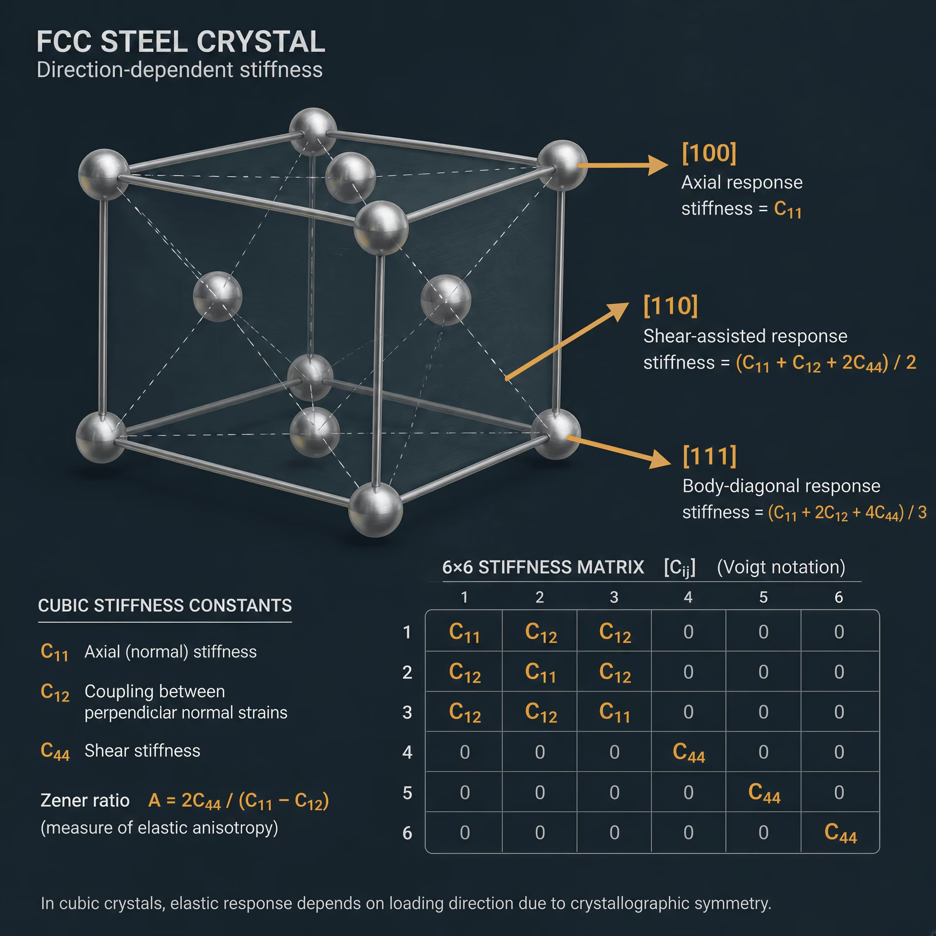
Elastic stiffness tensors in cubic crystals
Linear elasticity relates stress to strain through a fourth-order stiffness tensor:
The tensor contains the elastic stiffnesses , while its inverse contains the elastic compliances . Crystal symmetry reduces the number of independent terms. A completely general anisotropic solid can require 21 independent elastic constants, but a cubic crystal requires only three: , , and .
In contracted matrix notation, the cubic stiffness matrix is
\[ \begin{bmatrix} \sigma_1\\ \sigma_2\\ \sigma_3\\ \sigma_4\\ \sigma_5\\ \sigma_6 \end{bmatrix} = \begin{bmatrix} C_{11}&C_{12}&C_{12}&0&0&0\\ C_{12}&C_{11}&C_{12}&0&0&0\\ C_{12}&C_{12}&C_{11}&0&0&0\\ 0&0&0&C_{44}&0&0\\ 0&0&0&0&C_{44}&0\\ 0&0&0&0&0&C_{44} \end{bmatrix} \begin{bmatrix} \varepsilon_1\\ \varepsilon_2\\ \varepsilon_3\\ \varepsilon_4\\ \varepsilon_5\\ \varepsilon_6 \end{bmatrix}. \]
The three constants have different roles. describes a normal stress response along a cubic axis, couples normal deformation between perpendicular axes, and describes a shear response on a principal crystallographic plane. They are stiffnesses, not interchangeable versions of Young’s modulus or shear modulus.
A useful cubic-crystal anisotropy indicator is the Zener ratio,
When , the cubic elastic response has the same directional form as an isotropic solid. Values away from one indicate orientation dependence. The ratio does not by itself give the modulus of a steel product; it describes the elastic symmetry of a crystal when the relevant single-crystal constants have been measured or calculated.
The NIST monocrystal chapter, published in 1982, shows how these stiffness data can be converted into aggregate properties for cubic and hexagonal materials. For a cubic crystal, the bulk modulus associated with uniform hydrostatic strain is
This is consistent with the thermodynamic definition reported by NIST,
The shear and Young’s moduli of a single crystal still depend on direction, even though the hydrostatic bulk response of a cubic crystal is symmetry-constrained. A direction such as , , or can produce a different tensile modulus because the applied stress resolves differently against the lattice.
For an isotropic material, only two elastic constants are independent, as described by Springer’s Elasticity of Solids chapter in 2020. Sandia’s Sierra documentation lists the related isotropic set as Young’s modulus , Poisson’s ratio , bulk modulus , shear modulus , Lamé’s first parameter , and ; any two suitable members determine the rest. That reduction does not apply to a crystal merely because the crystal is small or because its deformation remains elastic. It follows from isotropic symmetry.
Texture and directional modulus
A crystal orientation is commonly expressed by its crystallographic direction and plane relative to the specimen axes. In a polycrystalline sheet, the orientation distribution function records how grain orientations are distributed. Texture develops when processing favors particular lattice rotations, especially during rolling, recrystallization, and subsequent phase transformation.
The measured tensile modulus in the rolling direction therefore need not equal the modulus transverse to rolling or through the sheet thickness. The difference results from the orientation-weighted sum of grain responses, not from a new independent “rolling-direction Young’s modulus” that replaces the underlying stiffness tensor. A finite-element model can represent this behavior by assigning an anisotropic stiffness tensor to the material coordinates, or by assigning crystal-level properties to many orientations.
Rolled low-carbon steel, ferritic stainless steel, and transformation-processed sheet may show texture from deformation and recrystallization. Forged steel can develop direction-dependent grain flow and texture around the forging axis. Cast steel often has a more varied orientation distribution, but solidification can still produce columnar grains, segregation, phase gradients, or preferred orientations. None of these processing routes guarantees either isotropy or a particular magnitude of anisotropy.
Additively manufactured steel presents another orientation problem. Layer-by-layer thermal cycling can produce columnar grains aligned with a build direction, while scan strategy, melt-pool geometry, reheating, and heat treatment alter the orientation distribution and phase constitution. A modulus measured parallel to the build direction may consequently differ from one measured transverse to it. The direction, specimen location, heat treatment, porosity, and test method must accompany the reported value.
Texture also affects Poisson’s ratio and shear modulus. A tensile test may report an axial strain response, while a resonant method infers several dynamic constants from vibration modes. ASTM E1875-20a specifies determination of dynamic Young’s modulus, shear modulus, and Poisson’s ratio “by sonic resonance.” Those dynamic values are not automatically identical to static values from a slow tensile test, particularly when damping, microcracking, porosity, temperature, or frequency affects the response.
Quasi-isotropic polycrystalline estimates
When grain orientations are sufficiently dispersed, directional differences may average to small values at the specimen scale. Engineers then describe the aggregate as quasi-isotropic: not perfectly isotropic at every grain or local volume, but adequately represented by isotropic constants for the intended calculation. The word matters. It identifies an approximation, not a claim that all crystallographic anisotropy has disappeared.
Polycrystalline estimates can be formed from single-crystal stiffness or compliance data using bounds and averaging schemes. A Voigt estimate assumes a uniform strain across grains; a Reuss estimate assumes a uniform stress. Their predictions generally differ because neither condition exactly represents every heterogeneous aggregate. The Hill estimate, commonly taken as the arithmetic mean of the Voigt and Reuss results, often serves as a practical intermediate approximation. These estimates require a specified crystal symmetry, orientation distribution, and phase constitution.
For a quasi-isotropic aggregate, the resulting , , , and obey the familiar isotropic relationships:
and
Thus, once two independent aggregate constants are selected, the others are derived. A reference table may list an approximate bulk modulus of 163 GPa for stainless steel, as Engineering ToolBox did in 2024, but that figure is a secondary estimate rather than a universal value for every stainless-steel grade, temperature, product form, phase balance, or measurement method.
The National Bureau of Standards report on Fe-5Cr-26Mn austenitic steel illustrates the measurement issue directly: elastic constants were determined over 76–400 K from longitudinal- and transverse-mode sound velocities. Temperature changes lattice spacing, phase stability, defect mobility, and wave velocity, so the resulting constants describe specified test conditions. For design, a quasi-isotropic set may be appropriate for a cast or annealed product with weak texture. A strongly rolled sheet, forged component, weld, or additively manufactured build may require directional data instead. The correct modulus is therefore not simply the number attached to a steel grade; it is the value associated with the deformation mode, orientation, temperature, microstructure, and test method.
How Steel Elastic Constants Are Measured
Steel elastic constants are measured either from a force–displacement response or from the propagation and resonance of mechanical waves. These approaches do not always produce the same numerical modulus. A tensile test records a near-static slope under a particular loading rate, while sonic and ultrasonic methods measure a high-frequency, small-amplitude response. Temperature, grain structure, crystallographic texture, porosity, phase constitution, residual stress, specimen geometry, and the definition of the measured mode can all affect the result.
For an isotropic, linear elastic solid, only two elastic constants are independent. Young’s modulus , shear modulus , bulk modulus or , Poisson’s ratio , Lamé’s first parameter , and describe related aspects of the same constitutive response; Sandia National Laboratories lists this set and states that and determine the others. The measurement method therefore matters even when the reported quantities have familiar names. Young’s modulus describes axial extension, bulk modulus describes volume change under hydrostatic pressure, and shear modulus describes angular distortion.
Mechanical tensile and compression methods
The conventional tensile method determines a static or quasi-static Young’s modulus from the slope of the initial linear part of a stress–strain curve:
A machined steel specimen is loaded in tension while an extensometer, strain gauge, or optical system measures axial strain. The useful slope is taken before plasticity, Lüders deformation, cracking, or other non-linear behavior begins. The selected strain interval must be stated because small deviations from linearity, machine compliance, seating effects, and strain-resolution limits can change the fitted value.
A tensile test can also determine Poisson’s ratio by measuring the simultaneous lateral strain:
The axial and transverse measurements must be synchronized and taken in the same elastic interval. Once and are known, isotropic relations give
and
These calculated values are not separate measurements of shear or volumetric stiffness. They inherit the temperature, strain-rate, texture, and test-direction dependence of the original tensile data.
Compression testing provides another route to an axial modulus, but it introduces different errors. The specimen must be short enough to avoid buckling, yet long enough to provide a measurable displacement. End friction can restrain lateral expansion and produce a barreled specimen, so the measured force–displacement slope may include friction and platen alignment effects. Lubrication, end parallelism, surface finish, platen stiffness, and the ratio of specimen height to diameter all matter. Extensometers or displacement sensors should measure deformation over the specimen gauge length rather than relying only on crosshead travel.
Hydrostatic compression is conceptually closer to a direct bulk-modulus measurement because it applies pressure in all directions and tracks volume change:
This is the thermodynamic definition given by the National Institute of Standards and Technology in 1982. Ordinary uniaxial compression is not hydrostatic compression; it combines axial and lateral deformation and therefore does not directly measure . Direct bulk-modulus work requires pressure vessels, accurate volume or strain measurement, pressure calibration, and control of temperature. For most structural steel characterization, is instead calculated from independently measured and , or obtained from sound velocities.
Static mechanical slopes are particularly sensitive to test rate and specimen condition. A tensile result from a polished, stress-relieved bar tested at room temperature is not automatically the modulus of a textured rolled plate, a weld metal, or a two-phase heat-treated product. In a cubic single crystal, stiffness varies with crystallographic direction. A polycrystalline aggregate may appear quasi-isotropic when grains are randomly oriented, but rolling or solidification texture can leave direction-dependent moduli.

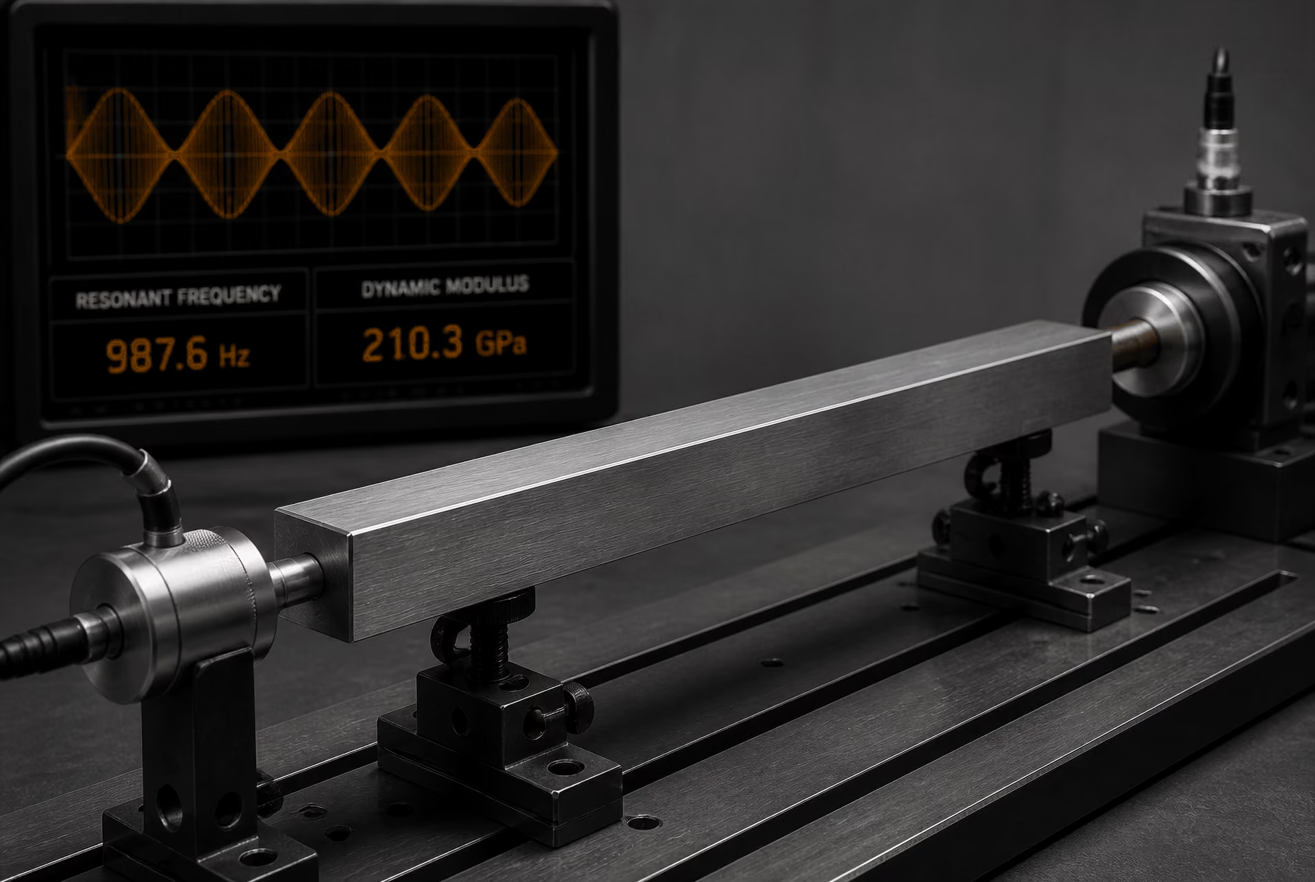
Sonic resonance under ASTM E1875-20a
ASTM E1875-20a is a named standard for determining dynamic Young’s modulus, shear modulus, and Poisson’s ratio “by sonic resonance.” Instead of measuring a long, slow force–strain slope, the method excites a specimen and identifies its natural resonant frequencies. The frequency at resonance depends on elastic stiffness, mass density, specimen dimensions, and the mode shape.
The specimen is supported in a way that approximates a free boundary condition, commonly by placing supports near nodal regions so that they remove as little vibrational energy as possible. A driver produces vibration, and a microphone, accelerometer, laser instrument, or another detector records the response. The resonant frequency is identified from a sharp amplitude maximum, a phase change, or a frequency-response peak. The measured frequency must be assigned to the correct flexural, torsional, or longitudinal mode; confusing adjacent modes can produce a plausible but incorrect modulus.
Specimen length, width, thickness, mass, and density are therefore central inputs. The dimensions should be measured at the test temperature when thermal expansion is significant, or corrected from room-temperature dimensions using an appropriate expansion coefficient. Density should correspond to the actual specimen rather than an assumed handbook value, especially for cast steel, porous material, particulate inclusions, or multiphase microstructures. ASTM E1875-20a incorporates specimen geometry and resonance equations rather than treating every sample as an infinite rod. End conditions, support location, aspect ratio, damping, and geometric corrections influence the calculated dynamic constants.
A torsional resonance primarily supplies shear information, while a flexural or longitudinal resonance supplies a modulus related to axial stiffness. Combining the dynamic and values permits calculation of
provided the isotropic linear-elastic assumption is appropriate. The resulting Poisson’s ratio is a dynamic value at the test frequency. It should not be presented as a universal grade constant independent of frequency or temperature.
Temperature control is part of the measurement, not an afterthought. The furnace or environmental chamber must bring the specimen to a stable, known temperature, and the resonance identification must account for thermal expansion, changing density, and the temperature dependence of stiffness. A frequency measured while the specimen is still warming does not represent a well-defined elastic state. Boundary conditions also change with temperature if supports expand, soften, slip, or alter contact pressure.
Longitudinal and transverse sound velocities
Ultrasonic measurements determine elastic constants from wave speeds. A longitudinal wave produces particle motion parallel to propagation; a transverse or shear wave produces particle motion perpendicular to propagation. For a homogeneous isotropic solid with density , the ideal relations are
and
Thus,
and
Poisson’s ratio can then be obtained from and , or directly from the velocity ratio under the same isotropic assumption. These equations are simple, but the measurements are not. The transit distance must be known accurately, echoes must be correctly assigned, and the transducer must generate and detect the intended polarization. An apparent longitudinal arrival can include mode conversion, surface waves, reflections, or dispersion.
A National Bureau of Standards report published in 1981 used longitudinal- and transverse-mode sound velocities to determine elastic constants for Fe-5Cr-26Mn austenitic steel over 76–400 K. That temperature range is important: it shows that elastic constants are measured functions of thermal state, not fixed labels attached to the alloy designation. The report’s procedure depended on controlled temperature, known density, defined specimen geometry, and reliable identification of both wave modes. Applying the room-temperature equations at cryogenic or elevated temperature without updating these quantities would obscure the actual temperature dependence.
Engineering ToolBox gives an approximate bulk modulus of 163 GPa for stainless steel. Limited evidence
The same caution applies to engineering reference tables. Engineering ToolBox gives an approximate bulk modulus of 163 GPa for stainless steel, but that figure is a secondary reference estimate, not a universal value for every stainless-steel grade, product form, texture, phase balance, temperature, or test method. A measured dynamic value for austenitic Fe-5Cr-26Mn, a static value from a tensile coupon of a ferritic grade, and a calculated value inferred from and answer different experimental questions. Reporting the method, specimen dimensions, density, temperature, resonance or wave mode, and boundary conditions is therefore as important as reporting the modulus itself.
Temperature, Phase, Composition, and Processing Effects
Steel elastic constants are not fixed labels attached permanently to a grade. They describe a material state, a deformation mode, and a measurement condition. Temperature, phase constitution, composition, crystallographic texture, porosity, inclusions, residual stress, and thermal history can all change the measured response. Strength may change by hundreds of percent across a transformation or tempering treatment while Young’s modulus changes by a much smaller proportion, but “smaller” does not mean negligible in precision analysis.
For an isotropic linear-elastic solid, only two elastic constants are independent. Young’s modulus , shear modulus , bulk modulus or , Poisson’s ratio , Lamé’s first parameter , and are related quantities, as described by Springer’s Elasticity of Solids and Sandia National Laboratories’ Sierra documentation. If temperature or microstructure changes one independent constant, the others calculated from it must be updated consistently. A reported modulus therefore needs a temperature, product condition, direction, and test method attached to it.
Temperature dependence of elastic constants
Elastic stiffness usually decreases as temperature rises. Atomic vibrations increase, interatomic bonds become less resistant to small displacement, and thermal expansion changes the equilibrium spacing between atoms. The effect is often gradual within a single phase, although magnetic transitions, recovery, recrystallization, and phase transformations can introduce sharper changes. Near a transformation temperature, a single room-temperature value is especially poor as a substitute for a temperature-dependent material model.
The National Bureau of Standards report on Fe-5Cr-26Mn austenitic steel provides a useful example. Published in 1981, it determined elastic constants between 76 and 400 K from longitudinal- and transverse-mode sound velocities. This is a dynamic measurement: the wave speeds provide the longitudinal and shear stiffnesses, from which related constants can be calculated. The result demonstrates that even an austenitic steel retained over the test interval does not possess one temperature-independent set of elastic constants. The temperature interval extends from cryogenic conditions to above room temperature, so the measured values describe a curve, not a single grade property.
The distinction between strength and stiffness matters here. Yield strength can rise strongly at low temperature because dislocation motion becomes more difficult, while the elastic slope changes less dramatically. Conversely, a small change in can alter predicted deflection, buckling load, contact pressure, or thermal-stress partitioning. Plastic strength and elastic stiffness answer different questions. A steel can become much stronger without becoming proportionally stiffer.
Dynamic and static tests may also produce different reported values. ASTM E1875-20a specifies determination of dynamic Young’s modulus, shear modulus, and Poisson’s ratio by sonic resonance. Resonance tests operate at small strain and high frequency, whereas a tensile test obtains a static or quasistatic slope over a prescribed strain interval. Microplasticity, anelasticity, instrument compliance, specimen geometry, surface condition, and frequency can influence the comparison. Neither result should be treated as universally interchangeable with the other.
Bulk modulus has a distinct physical meaning: it measures resistance to volumetric compression. NIST defines it thermodynamically as . Engineering ToolBox lists an approximate bulk modulus of 163 GPa for stainless steel, but that figure is a secondary reference estimate, not a universal value for every stainless-steel grade, temperature, product form, phase constitution, or test condition. The same caution applies to tabulated , , and .
Austenite, ferrite, martensite, and multiphase steels
Phase constitution affects elastic response because each phase has its own crystal structure, composition, lattice parameter, magnetic state, defect population, and single-crystal stiffness tensor. Ferrite has a body-centred cubic structure, austenite a face-centred cubic structure, and martensite is commonly a body-centred tetragonal or highly distorted body-centred structure when carbon produces appreciable tetragonality. These labels do not specify one unique modulus. Carbon content, substitutional alloying, ordering, dislocation density, and retained defects alter the stiffness of each phase.
Austenitic steels provide a clear warning against assigning a generic “austenite modulus.” The Fe-5Cr-26Mn study examined a particular chemistry and temperature range, not every Fe-Cr-Mn alloy or every steel described as austenitic. Manganese and chromium affect lattice stability and magnetic behaviour, while temperature can alter magnetic order even when the crystal structure remains austenitic. Such changes influence interatomic forces and therefore elastic constants.
Ferritic steels can show temperature-dependent elastic behaviour associated with their ferromagnetic state and its transition toward paramagnetism. The change need not coincide with a visible phase transformation. Martensitic steels add another layer: quenching creates supersaturation, high dislocation density, internal stresses, and often carbon-dependent tetragonality. Tempering then causes carbide precipitation, recovery, and redistribution of carbon. The elastic response measured after tempering is therefore not simply the response of an ideal martensite crystal.
Multiphase steels require an effective-property interpretation. In ferritic-martensitic, dual-phase, bainitic, or retained-austenite-containing steels, an apparent modulus reflects phase fractions, phase connectivity, crystallographic orientation, interfaces, porosity, and the direction and scale of the test volume. A rule-of-mixtures estimate may provide a first approximation, but local constraint means that phases do not all carry the same strain or stress. A stiff martensitic region embedded in ferrite can alter the measured slope through load transfer, while retained austenite may transform during loading and make the response depart from linear elasticity.
At the single-crystal level, cubic and hexagonal crystals have direction-dependent stiffnesses. Polycrystalline steel approaches isotropy only when grain orientations are sufficiently random and the specimen contains enough grains for averaging. Rolled plate, strip, and bar may retain texture, producing different longitudinal, transverse, and through-thickness moduli. In that case, forcing one isotropic and one isotropic into a calculation can hide a real directional response.
Casting, rolling, heat treatment, and residual stress
Processing changes both the intrinsic phase properties and the effective stiffness of the manufactured body. Cast steel can contain shrinkage porosity, gas pores, oxide films, segregation, dendritic structure, inclusions, and coarse or nonuniform grains. Even a small volume fraction of connected porosity can reduce the effective modulus more than a handbook value for fully dense steel would suggest. Inclusions may be stiff or compliant relative to the matrix, and poorly bonded inclusions act as stress concentrators or crack-like defects during a dynamic or static test.
Rolling refines and elongates grains, breaks up cast structure, and introduces crystallographic texture. The resulting elastic anisotropy may be modest for some products and significant for others. Reduction schedule, rolling temperature, recrystallization, and final thickness all matter. A modulus measured along the rolling direction should not automatically be assigned to the transverse or normal direction.
Heat treatment changes phase fractions, grain size, dislocation density, precipitates, carbide morphology, and retained stress. Normalizing can refine a ferrite-pearlite structure; quenching can create martensite and residual stress; tempering reduces some of that stress while changing precipitation and recovery. Annealing may reduce dislocation density and texture-related effects through recrystallization. These treatments can produce substantial changes in yield strength and toughness while leaving the small-strain modulus comparatively close to its prior value, though the measured effective modulus can still shift through defects, phase transformation, or texture.
Residual stress deserves separate treatment. A self-equilibrated stress field does not necessarily change the ideal tangent modulus of a flawless, homogeneous, linear-elastic crystal. It can, however, change what an experiment records. Residual stress alters wave propagation, specimen curvature, contact conditions, crack closure, and the onset of microplasticity. In a tensile test, an apparent initial slope may be affected by straightening, grip alignment, stress redistribution, or incomplete removal of machining stresses. In resonance testing, stress and anisotropy can shift natural frequencies.
Consequently, a defensible steel modulus statement identifies the phase condition, thermal state, product direction, density or defect condition, and measurement method. The number is a property of that defined state—not a permanent grade constant.
Steel Grade Designations and Responsible Property Tables
A steel designation identifies a composition, product class, or specification requirement; it does not, by itself, provide a complete elastic-property record. “304 stainless steel,” “AISI 1045,” and “ASTM A572 Grade 50” are useful material references, but none of those names alone states the product form, thermal history, crystallographic texture, test temperature, or method used to obtain an elastic modulus.
That distinction matters because isotropic linear elasticity has only two independent constants. The set commonly reported in engineering includes Young’s modulus , Poisson’s ratio , bulk modulus or , shear modulus , Lamé’s first parameter , and . Sandia National Laboratories states that and determine the remaining constants when isotropic relations apply. OpenStax assigns different physical meanings to the principal moduli: describes tensile or uniaxial response, describes volumetric compression, and describes shear deformation. A table that presents four apparently independent numbers without explaining their source can therefore imply a precision or independence that the material model does not possess.
Austenitic, ferritic, martensitic, and precipitation-hardening stainless steels
Stainless-steel family names describe metallurgical structure, not one universal elastic response. Austenitic grades such as Type 304, Type 304L, Type 316, and Type 316L are commonly identified under ASTM product specifications by the relevant “Type” designation and, where applicable, by UNS numbers such as UNS S30400, UNS S30403, UNS S31600, and UNS S31603. The designation must be reproduced as written in the applicable standard. “304L stainless” should not silently be converted into “304,” because the low-carbon grade has a different composition requirement and may receive different processing.
Ferritic grades include Type 430 and Type 409, while martensitic grades include Type 410, Type 420, and Type 440C. These names identify families with different phase stability, carbon levels, alloy additions, hardening response, and magnetic behavior. Their elastic properties can be affected by cold reduction, annealing, quenching, tempering, retained austenite, carbide populations, and the direction of measurement. A forged or rolled product may not behave like a cast product carrying a chemically similar designation.
Precipitation-hardening stainless steels require still greater care. 17-4 PH is a widely used designation, but a specification may identify the material as UNS S17400 and define conditions such as H900, H1025, or H1150. Those condition designations are heat-treatment states, not interchangeable grade names. A property table listing “17-4 PH modulus” without stating the condition leaves a significant part of the material description missing. The matrix, precipitate state, residual stress, and prior deformation can differ between conditions even when the nominal alloy designation remains unchanged.
The ASM Steel Castings Handbook treats modulus of elasticity, Poisson’s ratio, shear modulus, and related physical properties as steel-casting data. That framing is important: a cast-steel table describes a specified casting material and test basis, not every wrought, welded, additively manufactured, or heat-treated product with a similar chemistry. Castings may contain segregation, porosity, inclusions, and local microstructural variation that affect measured results and their scatter.
Nor should stainless family labels be used to assign a single exact modulus. An approximate secondary reference value of 163 GPa for stainless steel appears in Engineering ToolBox, but that figure is not a universal value for every stainless grade, temperature, product form, or test condition. It is a reference estimate, not a substitute for a standard-specific data sheet or a measured value.
Carbon and low-alloy steel designations
Carbon and low-alloy steels also require exact designation practice. AISI/SAE 1045 identifies a carbon steel in the SAE/AISI numbering system; it is not the same designation as ASTM A36, which is a product specification for structural steel. ASTM A572 Grade 50 identifies a grade within ASTM A572/A572M, while AISI/SAE 4130 identifies a chromium-molybdenum alloy steel composition. These labels should not be merged into informal forms such as “4130-grade A572” unless a governing specification explicitly supports that description.
European designations provide another example. S355J2 and S355JR are designations used within EN 10025-2, and the suffixes carry specified impact-test or delivery-condition meaning. They are not merely alternative names for ASTM A572 Grade 50. Chemical similarity does not establish equivalence of specification requirements, product dimensions, inspection rules, or elastic-property data.
A table should also distinguish a composition designation from a delivery condition. AISI/SAE 4140 may be supplied annealed, normalized and tempered, quenched and tempered, forged, or in another specified condition. ASTM A36 plate, bar, and structural shapes are governed by a product specification, but their measured response can still depend on thickness, rolling direction, residual stress, and test method. The nominal grade sets limits or requirements; it does not erase manufacturing history.
The same caution applies to “mild steel,” “tool steel,” “high-strength low-alloy steel,” and similar family descriptions. These are broad categories, not complete grade designations. A responsible table gives the standard number, grade or type, revision where relevant, UNS or AISI/SAE designation when applicable, product form, and heat-treatment condition. If a designation is an internal company name, it should be marked as such rather than presented as an ASTM, ASME, SAE, AISI, EN, or UNS designation.
Why standards and product specifications must accompany values
Elastic-property values are meaningful only with their measurement context. At minimum, a table should identify:
- the product form: plate, sheet, bar, tube, wire, forging, weld metal, powder-processed part, or casting;
- the heat treatment and condition, including temper, aging, solution treatment, or precipitation-hardening state;
- the test direction relative to rolling, forging, extrusion, or build direction;
- the temperature and environmental condition;
- the loading rate or frequency;
- the specimen geometry and relevant dimensions;
- the test standard and revision;
- whether the result is static, quasi-static, or dynamic;
- the number of specimens, range, mean, and scatter where available.
Static and dynamic moduli are not automatically interchangeable. ASTM E1875-20a specifies determination of dynamic Young’s modulus, shear modulus, and Poisson’s ratio “by sonic resonance.” Resonance measurements use wave propagation and vibration frequency, whereas a tensile test can determine a slope from a stress–strain curve under a defined loading rate. Both methods concern elastic response, but they can produce different reported values because frequency, damping, microstructural defects, instrumentation, and data-reduction procedures differ.
Temperature must be stated, especially for cryogenic or elevated-temperature work. A 1981 National Bureau of Standards report measured elastic constants for Fe-5Cr-26Mn austenitic steel over 76–400 K using longitudinal- and transverse-mode sound velocities. That range demonstrates why a room-temperature value cannot be copied into a cryogenic design table without qualification. Texture and crystal anisotropy add another issue: the NIST handbook chapter on monocrystal elastic constants explains how quasi-isotropic polycrystalline , , , longitudinal modulus, and can be derived from single-crystal stiffness data, but such derivations depend on crystal symmetry, orientation distribution, and averaging assumptions.
For isotropic calculations, one carefully identified pair of constants is enough; the others should be calculated with the stated equations or checked for consistency. For anisotropic rolled, forged, textured, welded, or additively manufactured steel, a single scalar modulus may be an approximation rather than a complete constitutive description. Standards and product specifications prevent a table from disguising that limitation. They connect each number to a defined material, condition, direction, temperature, and method—the information needed before the value can responsibly enter a design calculation.
Design Use: Selecting the Correct Modulus Relationship
An elastic modulus belongs to a deformation mode. Young’s modulus describes the normal strain produced by uniaxial stress; shear modulus describes distortion at nearly constant volume; and bulk modulus , also written , describes resistance to uniform compression. Poisson’s ratio connects normal and lateral strain. These quantities are related, but they are not interchangeable merely because they are all reported in gigapascals or are commonly listed together for steel.
For a homogeneous, linear, isotropic solid, only two elastic constants are independent. Springer’s Elasticity of Solids states this directly in its 2020 treatment of isotropic elasticity. Sandia National Laboratories lists the associated set as Young’s modulus , Poisson’s ratio , bulk modulus , shear modulus , Lamé’s first parameter , and , with and determining the others. The conversion equations are therefore conditional relationships, not independent measurements of six unrelated material properties:
and
The assumptions matter. These equations apply to small strains, linear elastic response, and isotropic behavior. A steel plate with rolling texture, a weld heat-affected zone, a cast product containing directional solidification, or a two-phase microstructure may not meet the isotropic assumption closely enough for one converted value to represent every loading direction.
Uniaxial members and E
For a straight tension member, compression member, tie, rod, or slender beam segment under an axial force, is the primary modulus. The basic relation is
so the elastic extension of a prismatic member is
where is axial force, is original length, and is cross-sectional area. This is the correct starting point for estimating elastic elongation, shortening, and axial stiffness .
Poisson’s ratio enters when lateral contraction or multiaxial constraint matters. A freely stretched steel bar contracts laterally according to
For a fully constrained specimen, however, the axial response is not represented by alone. Lateral strain cannot develop, so the stress state becomes three-dimensional and the apparent stiffness rises. A finite-element model of a bonded insert, a constrained washer, or a press fit must account for this coupling rather than treating the component as an isolated one-dimensional bar.
The value used for must also match the measurement and service condition. A static tensile-test slope, a resonant dynamic modulus, and a modulus inferred from ultrasonic velocity can differ because of frequency, temperature, specimen geometry, porosity, residual stress, and defects. ASTM E1875-20a specifies determination of dynamic Young’s modulus, shear modulus, and Poisson’s ratio “by sonic resonance.” That method does not automatically produce the same number as a slow tensile test at the design temperature.
Steel is not one elastic material in every metallurgical state. Ferritic, martensitic, bainitic, and austenitic structures can differ, while texture can make the rolling direction and transverse direction respond differently. The National Bureau of Standards report on Fe-5Cr-26Mn austenitic steel determined elastic constants from longitudinal- and transverse-mode sound velocities over 76–400 K. That temperature range is a reminder that an elastic constant measured near room temperature should not be treated as temperature-independent data for cryogenic or elevated-temperature service.
Torsion and G
For a circular shaft in elastic torsion, controls the angle of twist:
where is torque, is the polar second moment of area, and is shaft length. The torsional stiffness is . The associated shear stress in a circular shaft is
Using directly in this calculation gives the wrong stiffness unless it is first converted through a defensible value of . For isotropic steel,
That conversion is useful when only and are available, but it does not make a tensile measurement a direct torsional measurement. A material may show direction-dependent shear response even when an averaged tensile modulus appears acceptable.
The distinction becomes important for thin-walled tubes, splines, welded shafts, and parts with anisotropic manufacturing histories. In a general section, torsion may produce warping and a nonuniform shear field, so Saint-Venant’s circular-shaft equation may itself be insufficient. The material input is still a shear constitutive parameter, but the section analysis must represent the actual geometry.
Dynamic shear data require similar care. Resonance methods measure response at a particular frequency and small strain amplitude. A value calculated from a sonic test may be suitable for vibration or wave analysis, yet not identical to the secant or tangent stiffness used in a slow-load structural calculation. The designation “dynamic” is not a minor label; it identifies a different experimental condition.
Hydrostatic, contact, and wave problems
Bulk modulus or is the appropriate parameter for volumetric response. Under hydrostatic pressure, pressure changes volume according to
the thermodynamic definition given by the National Institute of Standards and Technology in 1982. A high means that substantial pressure produces only a small fractional volume change. This is different from resistance to shape change, which is governed mainly by .
Engineering ToolBox gives an approximate bulk modulus of 163 GPa for stainless steel. That figure can serve as a secondary reference estimate, not as a universal value for every stainless-steel grade, temperature, product form, phase constitution, or test method. Since , small errors in can produce a noticeable change in the calculated bulk modulus when approaches 0.5.
Contact calculations require both normal and tangential behavior. In Hertzian contact, the effective normal modulus for two bodies is commonly written
\[ \frac{1}{E^*} = \frac{1-\nu_1^2}{E_1} + \frac{1-\nu_2^2}{E_2}. \]
Here \(E^*\), not for one steel grade alone, controls the local elastic indentation. Frictional sliding and tangential traction introduce and as well. A model that substitutes for \(E^*\) may remain mathematically stable and produce smooth contact pressures, yet represent the wrong deformation mechanism.
Wave problems use still another combination. For an isotropic solid, the longitudinal wave modulus is
with longitudinal and shear wave speeds
\[ v_L=\sqrt{\frac{K+4G/3}{\rho}}, \qquad v_S=\sqrt{\frac{G}{\rho}}. \]
Thus, longitudinal velocity alone does not identify every elastic constant; a transverse-wave measurement is needed to separate and . In a single crystal or textured polycrystal, wave speed also depends on propagation direction and polarization, so isotropic formulas can conceal real elastic anisotropy.
Three-dimensional finite-element formulations generally use and , and , or Lamé parameters and . The choice is mathematical, not a change in physical material. Near incompressibility, however, an - formulation with close to 0.5 can suffer volumetric locking, while a mixed formulation using pressure and deviatoric response may perform better. Conversely, inserting independently rounded , , and values can violate the isotropic conversion equations and create an internally inconsistent stiffness matrix.
That is the central design risk: a converted constant may be numerically consistent with an equation while being physically inappropriate for the problem, temperature, frequency, direction, or steel microstructure being modeled. Select the modulus from the deformation mode first, then verify that its measurement conditions and isotropic assumptions match the component and analysis.
Common Errors in Steel Modulus Calculations
Steel modulus calculations often fail because quantities with different physical meanings are treated as interchangeable. Young’s modulus , shear modulus , bulk modulus or , and Poisson’s ratio describe elastic deformation. Yield strength describes the onset of substantial permanent deformation. They belong to different parts of a material model.
For an isotropic, linear-elastic solid, only two elastic constants are independent. Springer’s Elasticity of Solids chapter (2020) states this directly. Sandia National Laboratories lists the related set as Young’s modulus , Poisson’s ratio , bulk modulus , shear modulus , Lamé’s first parameter , and ; specifying and determines the others. Common conversions are
and
Those equations are not independent experimental facts. They are consequences of the isotropic linear-elastic assumption. Their use requires compatible values, consistent units, and a material state for which isotropy is a reasonable approximation.
Confusing modulus with yield strength
Common calculation errors
- Strength substitution Using yield strength in place of Young’s modulus confuses a plastic limit with elastic stiffness.
- Unit mixing Combining MPa and GPa without conversion can introduce a factor-of-1000 error.
- Method mixing Combining static E with dynamic ν or G can create an algebraically valid but physically inconsistent set.
- Direction omission Using one scalar modulus for strongly textured plate, wire, welds, or additively manufactured material can hide anisotropy.
- Temperature omission Applying one room-temperature value to cryogenic or elevated-temperature service can misrepresent the response.
The most persistent error is calling a high-strength steel “stiffer” because its yield strength is higher. Yield strength measures the stress at which plastic strain begins according to a specified criterion, often a proof strain such as 0.2%. Young’s modulus measures the slope of the elastic stress–strain response before that transition. A heat treatment, cold-reduction schedule, precipitation reaction, or change in carbon content can raise yield strength substantially without producing a comparable change in the initial elastic slope.
This distinction matters in design. Deflection under a service load is governed primarily by , geometry, boundary conditions, and load; the allowable stress check also requires yield strength or another strength limit. Replacing with a grade’s yield strength produces dimensionally plausible but physically meaningless results. A calculation that divides stress by yield strength may estimate a utilization ratio. It does not calculate elastic strain.
The same mistake appears in shear. Shear modulus is defined by the elastic relation between shear stress and shear strain,
Shear yield strength is a plastic limit. It may be estimated from a yield criterion, such as the von Mises relation, but it is not , and it is not obtained by assigning the units of stress to a modulus and changing its name. OpenStax (2020) separates the deformation modes clearly: Young’s modulus describes tensile response, bulk modulus describes volumetric compression, and shear modulus describes shear deformation.
A steel specification can therefore contain both a yield-strength requirement and an elastic-property assumption without those numbers being linked by a simple grade conversion. For structural calculations, the relevant designation and product standard should be recorded—for example, ASTM A240/A240M plate or sheet, EN 10025-2 S355 material, or ASTM A276 Type 304 stainless steel—along with thickness, product form, and test direction. The designation identifies the material requirement; it does not make a generic modulus value exact for every product.
Another error is treating every grade as having one exact . Ferritic, martensitic, bainitic, austenitic, and duplex steels can have different phase fractions, textures, porosity levels in cast products, and residual stresses. These factors affect measured elastic response. For many engineering estimates, a conventional isotropic value is adequate, but it remains an assumption or adopted design value, not a universal physical constant attached to the word “steel.”
Mixing static and dynamic values
Static and dynamic moduli are related but are not automatically interchangeable. A static modulus is obtained from a slowly applied mechanical test, commonly from the slope of a tensile or compression stress–strain curve over a stated strain interval. The result can be affected by machine compliance, grip alignment, surface condition, strain rate, hysteresis, microplasticity, and how the slope is fitted.
A dynamic modulus is inferred from wave propagation, resonance, or another time-dependent measurement. ASTM E1875-20a specifies determination of dynamic Young’s modulus, shear modulus, and Poisson’s ratio “by sonic resonance.” The specimen’s resonant frequencies and dimensions are used to infer elastic constants. This method can provide precise small-strain data, but the result corresponds to high-frequency, very small-amplitude deformation and should be labeled accordingly.
Dynamic measurements also depend on density, specimen geometry, frequency, temperature, and mode identification. A value derived from a longitudinal resonance should not be inserted into a shear calculation without the appropriate relation and a compatible Poisson’s ratio. Likewise, a handbook’s “modulus of elasticity” may be a design convention, while a resonance report may identify a dynamic modulus. The two should not be compared as though they came from the same test.
When converting between , , and , report whether the inputs are static or dynamic. Combining a tensile-test with a sonic-resonance can create an internally inconsistent set even when both numbers are individually credible. The calculation may satisfy the algebra while failing to represent a single measured material state.
Poisson’s ratio deserves special care because uncertainty in becomes important in the bulk-modulus equation. If GPa and , the isotropic relation gives GPa. If the same is combined with , GPa; with , it becomes GPa. A change of only 0.01 in changes the calculated by roughly 5%. Near , the sensitivity is much greater because approaches zero. Report the assumed value, its source, and a sensitivity range rather than presenting the resulting as a measured constant.
Units create a simpler but frequent failure. Since , an value entered in MPa alongside a value entered in GPa can introduce a factor-of-1000 error. Keep all moduli in one unit system through the calculation and state the unit beside the final result.
Bulk modulus values require provenance. Engineering ToolBox lists an approximate value of 163 GPa for stainless steel, but that is a secondary reference estimate, not a universal value for every stainless-steel grade, product form, temperature, or test condition. A defensible citation should identify the original measurement or calculation, composition, phase condition, temperature, pressure range, density basis, and method. The thermodynamic definition from the National Institute of Standards and Technology (1982), , makes the temperature condition explicit. A number copied from a table without those conditions should be marked approximate.
Ignoring anisotropy and temperature
The isotropic equations assume that the response is the same in every direction. Rolled plate, drawn wire, forged bar, and additively manufactured steel commonly develop crystallographic texture. Their elastic response can vary with the loading direction even when the material appears uniform to the unaided eye. A strongly textured sheet may require direction-specific constants rather than one , , and .
Single-crystal elasticity is described by an elastic-stiffness matrix, not by one scalar modulus. NIST’s 1982 handbook chapter explains how quasi-isotropic polycrystalline constants can be derived from single-crystal stiffness data for cubic and hexagonal elements. That averaging is a model. It becomes less suitable when texture is strong, phase proportions vary spatially, or the product contains aligned inclusions or pores.
Temperature is another omitted variable. Elastic constants generally change with temperature, and phase transformations can produce larger discontinuities than ordinary thermal softening. A National Bureau of Standards report (1981) measured elastic constants for Fe-5Cr-26Mn austenitic steel from 76 to 400 K using longitudinal- and transverse-mode sound velocities. The temperature range itself shows why a room-temperature value cannot be transferred silently to cryogenic service or elevated-temperature equipment.
A calculation should therefore state the material designation, product form, test direction, temperature, deformation mode, measurement method, and whether the constants are static, dynamic, isotropic, or direction-specific. If those details are unavailable, label the result as an engineering estimate and show how uncertainty in , , , and affects the answer. That is more accurate than assigning one exact modulus to all steel and allowing an unstated assumption to control the design.
References
- [1] Bulk modulus definition. NIST handbook chapter, 1982. https://tsapps.nist.gov/publication/get_pdf.cfm?pub_id=851172
- [2] Standard Test Methods for Dynamic Young’s Modulus, Shear Modulus, and Poisson’s Ratio by Sonic Resonance. ASTM E1875-20a, 2020. https://www.astm.org/e1875-20a.html
- [3] Elasticity of Solids. Springer book chapter, 2020. https://link.springer.com/chapter/10.1007/978-3-030-44787-8_4
- [4] Stress, Strain, and Elastic Modulus. University Physics Volume 1, 2020. https://openstax.org/books/university-physics-volume-1/pages/12-3-stress-strain-and-elastic-modulus
- [5] Elastic Constants of Fe-5Cr-26Mn Austenitic Steel from 76 to 400 K. National Bureau of Standards report, 1981. https://www.govinfo.gov/content/pkg/GOVPUB-C13-3488bca643803d66b83ad6e7425b6724/pdf/GOVPUB-C13-3488bca643803d66b83ad6e7425b6724.pdf